


Next: The SAXS/GISAXS Interface
Up: The POWDER DIFFRACTION (2-D)
Previous: The CALIBRANT Command
The CAKE Command
The CAKE command is so called, because it allows an arbitrary
user ``cake'' of data to be defined, and integrated to one of a
large choice of single and multiple scans.
When the CAKE command is first entered, an initial ``cake''
is defined. First the beam centre is defined in the same manner as
the BEAM CENTRE command; see Section 11.4,
Page ![[*]](./crossref.png) . This is followed by graphical
input for the STARTING AZIMUTH, END AZIMUTH, INNER
LIMIT, and lastly the OUTER LIMIT. All these values expect the
OUTER LIMIT have defaults which may be used instead, by clicking
within the prompt boxes.
. This is followed by graphical
input for the STARTING AZIMUTH, END AZIMUTH, INNER
LIMIT, and lastly the OUTER LIMIT. All these values expect the
OUTER LIMIT have defaults which may be used instead, by clicking
within the prompt boxes.
The defined ``cake'' or integration area, will be drawn on top of the
image in inverse video. The CAKE sub-menu now appears. This is
shown in Figure 40. If the CAKE sub-menu is
exited, and re-entered within the same FIT2D session, the defined
``cake'' is remembered.
Figure 40:
The CAKE Sub-Menu
|
|
The following commands are available:
- EXIT: Exit CAKE sub-menu and return to calling menu.
- INTEGRATE: Integrate currently defined ``cake'' region, with
a choice of the number of azimuthal and radial/2-theta output
pixels. This allows enormous flexibility in defining intensity versus
azimuthal angle scans,
 scans, multiple scans, and
polar transformations.
scans, multiple scans, and
polar transformations.
- INNER RADIUS: Change inner radius/2-theta angle of the
currently defined ``cake'' integration region.
- ZOOM IN: Graphical region definition
- ?: List of available commands and short descriptions.
- END AZIMUTH: Change end azimuth of the
currently defined ``cake'' integration region.
- OUTER RADIUS: Change outer radial/2-theta angle of the
currently defined ``cake'' integration region.
- Z-SCALING: Automatic or user control of intensity display range;
see Section 5.3, Page .
- HELP: Detailed help text
- EXCHANGE: Swap current data with the ``memory''; see
Section 5.2, Page .
- START AZIMUTH: Change starting azimuthal angle of the
currently defined ``cake'' integration region.
- MASK: Mask or Un-mask data (masked pixels are not re-binned);
see Section 5.7, Page .
- BEAM CENTRE: Change beam centre, which defines the zero angle
for integration; see Section 11.4,
Page .
- FULL: Set ROI to be all of the currently defined data.
- UN-ZOOM: Zoom out to see more of the data
- ASPECT RATIO: Control automatic correct aspect ratio (or
not). After integration, the output is often highly non-square. For
better display it is often better to set AUTOMATIC CORRECT ASPECT
RATIO IMAGE DISPLAY to NO.
When a suitable ``cake'' has been defined and ``bad'' pixels masked out,
the INTEGRATION command should be selected. The TYPE OF
AZIMUTHAL/RADIAL OR 2-THETA TRANSFORM control form appears. An example
is shown in Figure 41.
Figure 41:
The TYPE OF AZIMUTHAL/RADIAL OR 2-THETA TRANSFORM Control Form
|
|
The following parameters may be controlled:
- START AZIMUTH: Change starting azimuthal angle of the
currently defined ``cake'' integration region.
- END AZIMUTH: Change end azimuth of the
currently defined ``cake'' integration region.
- INNER RADIUS: Change inner radius/2-theta angle of the
currently defined ``cake'' integration region.
- OUTER RADIUS: Change outer radial/2-theta angle of the
currently defined ``cake'' integration region.
- SCAN TYPE: Allows one of 4 different types
of integrated scans to be selected:
- 2-THETA: This is an equal angle scan,
equivalent to a scan on a
powder diffractometer. The scale is in
degrees.
- Q-SPACE:
This is similar to the 2-THETA
scan, but the output elements are in equal
Q-range bins. The scale is in inverse
nanometres.
The definition of Q is
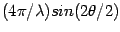 ,
where is the angle of the scattering as
recorded on the detector relative to the direct beam.
,
where is the angle of the scattering as
recorded on the detector relative to the direct beam.
- RADIAL: This is an equal radial distance
element scan. The scale is in millimetres.
- D-SPACINGS: This converts pixel angles to equivalent
D-spacings and outputs an scan in equal D-spacing distance pixels.
- AZIMUTH BINS: Number of bins in the output scan in the
azimuthal sense. This may be increased up to the size of the
program array in the second dimension.
- RADIAL BINS: Number of bins in the output scan in the
radial, , or Q-space sense. This may be increased up to
the size of the program array in the first dimension.
- CONSERVE INT.: NO means that the output
intensities are normalised by the number of
contributing pixels (although geometrical
corrections may be applied). This is appropriate
for producing the equivalent of a scan,
and for a Q-space scan, but does not converse
total intensity. For applications which require
integrated intensities to be conserved, this
should be set to YES.
- POLARISATION: YES to apply a polarisation
correction to the intensities during the
integration.
- FACTOR: This is the polarisation factor which
is used if the polarisation correction is
applied.
The polarisation factor is defined as
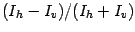 , where
  is the
horizontal component and
is the
horizontal component and  is the vertical
component. (Horizontal should normally
correspond to the X-direction of the image.)
is the vertical
component. (Horizontal should normally
correspond to the X-direction of the image.)
- DISTANCE: The sample to detector distance in millimetres.
- GEOMETRY COR.: YES corrects a flat ``scan'' to
the equivalent of a scan, or a Q-space
scan. (CONSERVE INT. should be set to NO). These are
the effect of change of distance and obliqueness
at higher angles for the flat image plate
compared to a detector on a arm, always
facing the sample.
By setting azimuthal bins to 1, a single 1-D radial//Q-space
scan can be obtained.
By setting the number of radial bins to 1, and selecting the ``cake''
as an annulus about a ring, or an arc peak, an integration of intensity
versus azimuth may be obtained.
Leaving both these numbers greater than 1, a 2-D polar transform is obtained.
In the output array the X-direction is used to store the
radial//Q-space bins and the Y-direction the azimuthal
bins10.
An example of the result of such a transform is shown in
Figure 42.
Figure 42:
Example of a Polar Transform of a Powder Pattern
|
|
Here the powder rings have become straight lines, at equal
angle. Any wobble in the lines shows inaccuracy in the beam centre, or
the detector tilt angles, or spatial distortion in the detector, or
maybe deviatoric stress
in the sample.
The black region at zero and low is the beam-stop shadow, and
the black regions at high are area outside the rectangular
input region.
Next: The SAXS/GISAXS Interface
Up: The POWDER DIFFRACTION (2-D)
Previous: The CALIBRANT Command
Andrew Hammersley
2004-01-09
![\includegraphics[width=17cm]{fit2d_cakemenu.ps}](img56.png)
![\includegraphics[height=22cm]{fit2d_cakeint.ps}](img57.png)
![\includegraphics[height=20cm]{fit2d_polartrans.ps}](img58.png)