
( 1)
Contents
Calulation of Potentials Using the Actual Crystal Structure
Mean square variation in path length
Calculation of the displacement correlation function
Muffin-tin Radii, and other Potential Parameters
Metallo-proteins - amino acids, Brookhaven files and torsion angles
Refinement of GE and I edges plus Xray diffraction pattern in RbGeIO6
RMC calculation of Co.8Mg.6Zn.6TiO4
12. Powder diffraction theory parameters
14. Fourier transform parameters
17. Restrained refinement parameters
19. Displacement correlation function parameters
The program was developed in the Chemistry Department of Southampton University in order to maximise the usefulness of the EXAFS technique in the investigation of crystalline materials which powder diffraction (PD) methods could not uniquely resolve.
The program retains many of the features of EXCURVE and provides most of the PD features of the program GSAS. For EXAFS this includes full multiple scattering calculations and whole-spectrum fitting, but at present it cannot deal with EXAFS polarisation dependence. PD calculations currently exclude calculation of the thermal diffuse scattering contribution, which is included in the background.
The command syntax and the manual closely follow EXCURVE. Indeed, this manual was the prototype of the new EXCURVE manual, and many features from this program have been incorporated into recent versions of EXCURVE. The program allows multiple edges, multiple phases and multiple oxidation states - phases may be amorphous, crystalline or small particles based on crystal lattices. The program may be used in EXAFS-only mode, but is unlikely to be useful as a diffraction-only program.
The purpose of the program is to find a structural model of a material which agrees with both the EXAFS spectra and PD profiles. As the program is primarily concerned with crystalline solids, the model is defined in terms of a unit cell, a space group and the positional coordinates of atoms. From this definition the cluster information required by EXAFS may readily be obtained. The information required consists of :
1. the radial or cartesian coordinates of scattering atoms about each absorbing atom for which spectra are available
2. a pair distribution function for each symmetrically unique excited-atom/scattering atom pair
3. the point group of each cluster
As the point symmetry and all the distances and angles within the structure are defined for each site, a full multiple scattering calculation may be performed to any required distance. The only information that cannot in principal be obtained from the crystallographic model is the displacement correlation function for each pair of atoms which allows the pair distribution functions to be calculated from the crystallographic thermal factors. This requires some additional input.
For amorphous solids, only the partial radial distribution functions for pairs of atoms are defined, and the calculation is in general limited to single scattering. Currently the contribution of non-crystalline phases to the diffraction pattern cannot be calculated.
The parameters used to define the model may be refined until optimum agreement with the XAFS and PD data is obtained.
Refinement may use additional data to that given by EXAFS spectra and PD profiles, for example distance and angle restraints using bond distances and angles obtained by other techniques.
The program can be used for both combined PD and EXAFS analysis, or else for either technique separately. For crystalline solids, the program is better suited than EXCURVE for EXAFS-only analysis, as it offers the option of refining either the positional or shell coordinates, and offers options such as Debye-temperature refinement for treatment of Debye-Waller factors. For PD-only refinements, however, it is not a suitable replacement for programs such as GSAS in most cases. It does not impose site-symmetry automatically, but relies on coupling between atomic coordinates to be defined. It is also far slower at refining due to the numerical methods used, although it eventually will usually give a better fit. It is however invaluable when the usual restrictions on symmetry need to be relaxed, in order to treat phenomena such as local lattice distotions or off-site displacement, which are hard to acheive with GSAS. The program is therefore ideally suited to the study of partially- or locally-ordered crystalline materials.
There are two modes of refinement - the first is similar to Excurve, and uses numerical estimates of the derivatives. It is slow but reliable, and can usually minimise any reasonably determined set of parameters. It can be used for all parameters, including phaseshift parameters. The second uses calculated derivatives with a Newton-Raphson minimisation. It may be faster, but is less stable, and cannot handle all parameters.
The manual is organised into a Theory section, a Program Guide, an Examples section, and Reference sections on Parameters and Commands, terminated by Tables. The program guide is largely a sequential guide, terminated by discussion of topics which might initially only be used optionally. Most of the background knowledge required is included in the theory section, but a basic knowledge of quantum mechanics is assumed, as is a knowledge of Unix or DOS commands, which can be used within the program to supplement the built-in commands. The reference sections contain definitions of the parameters and commands needed to analyze data, with information essential to their use but with a minimum of background material. References quoted in the text, together with others that might be useful, are given in the bibliography.
The small number of cases where the program is different to EXCURVE should be noted carefully. In particular, there are no ‘atom types’ in the EXCURVE sense. T parameters still exist, but use atomic numbers. Thus although the command
C T2 NA
Is the same for both programs, it is doing something different in each case.
Parameters indexed by atom-type in EXCURVE are here indexed by atomic number - thus MTR29 not MTR1 for a Cu central atom.
The command
C ATOM1
Is not used to define an atom type, but instead is a means of setting up positional coordinates (it is not normally used with an option number).
Acknowledgements.
I am grateful to the University of Washington, WA, and especially to Prof. J.Rehr for permission to use code derived from FEFF in calculating the Hedin-Lundqvist excited state exchange and correlation potential.
The refinement routine VA05A is used under licence from UKAEA, Harwell Laboratory.
This section discusses the calculation of the theoretical spectra, the way in which differences between theory and experiment are minimised, and the criteria used to define the best-fitting parameters.
Refinement involves minimising the quantity given by:
( 1)
The weightings wexafs etc. determine the relative significance of the EXAFS, distance, and angle contributions. The sum wexafs + wdistances + wangles must equal one.
Often, only the EXAFS contribution is used. The other two terms are restraints, used in special circumstances where a model includes well characterised groups of atoms.
The EXAFS contribution is given by:
( 2)
χexp(k) and χth(k) are experimental and theoretical EXAFS and:
( 3)
Here k is the magnitude of the photoelectron wavevector.
Similarly the powder diffraction contribution is:
( 4)
The distance and angle contributions to the refinement are:
( 5)
with:
( 6)
and:
( 7)
with:
( 8)
Where rref and rmodel refer to refined and model distances respectively, and where βref and βmodel refer to refined and model angles.
Calculation of the EXAFS theory
Analysis of XAFS spectra is greatly simplified by the fact that in a single particle approximation, provided coupling between final states is ignored, the atomic contribution (μ0) and the scattering contribution (χ) to the total absorption (μ) may be separated, as in:
( 9)
where the sum is over all allowed final states lm and the atomic contribution to the cross section, μ0lm (E) is given in the dipole approximation by the Golden rule expression:
(10)
Here e is the electric vector of the photon, r the position with respect to the atomic nucleus and D(E) the energy density of final states. D(E) depends on the way the wavefunctions are normalised and is usually 1 for Rydberg states below the ionisation threshold and proportional to k, the magnitude of the photo-electron wave vector for a free electron.
Unless otherwise stated, Hartree atomic units (h=e=m=1) are used to avoid unnecessary constants, hence the unit of μ is here the square of the Bohr radius.
Many-body effects may be included approximately within this basic formalism, for example by including additional terms for two-electron transitions, and by using effective one-electron potentials calculated for an embedded atom with a complex energy to account for inelastic losses to represent the true many body potential.
Until recently, it has been normal to separate the oscillatory part of the experimental spectrum, χ, from the atomic contribution by means of a background subtraction, in which the atomic background is approximated by polynomial or spline functions. Here it is assumed that this has been done, and it is only necessary to calculate the oscillatory part.
For an amorphous or polycrystalline sample, the oscillatory part of the spectrum due to a transition to a specific final state l is:
(11)
The final exponential factor is a phase term due to the outward and inward passage of the photoelectron through the central atom potential. It is described in terms of the atomic phaseshift δl, which is described later. The m sum is over all allowed quantum numbers -l ≥ m ≥ l.
Z is expanded as a scattering series:
(12)
Z1 includes a sum over all atoms, excluding the central atom, Z2 a sum over all pairs of atoms i ≠ j, etc.
For single scattering from an atom at (r,Ω):
(13)
Simple algebra leads to the well known expression of Gurman, Binsted and Ross:
(14)
The l sums are strongly restricted by the rules on coupling of angular momentum : (l1+l2+l) even, l2≤l1l, l1≥l2-l. This results in just two terms for a K-edge, 3 for an L3, etc. The 3J coefficient above is that of Brink and Satchler (1968), also given by Zare (1988).
The equation above refers to atoms in fixed positions r. Disorder is expressed as a pair distribution function g(r) describing the motion of a scattering atom relative to the central atom. In the case of static disorder, g(r) may also describe the distribution of an atom in a disordered site, again relative to the excited atom:
(15)
Where Z0 is calculated neglecting all thermal or static disorder. Traditionally this has been approximated by:
(16)
Here, even if Z is calculated exactly using a spherical wave theory, disorder is treated in a plane wave approximation, which ignores terms due to spherical-wave effects (see Rennert, 1992/3). This approximation gives rise to the familiar exponential Debye-Waller factor. This expression also ignores anharmonic contributions, that is the cumulant expansion of g(r) involves no terms of higher order than two. In this event, g(r) is a Gaussian characterised by σ:
(17)
Also ignored here are terms arising from motion of the atoms in the plane normal to the interatomic bond. The inclusion of these would give rise to multi-dimensional distribution function g(r). The treatment of disorder is discussed at greater length below.
For the single-scattering, polarisation independent expression above [13], all the structural information is included in the Hankel functions h(kr). Similarly all the information on the scattering atoms is contained within the T matrix, whose l'th element is given by:
(18)
Here it is assumed that T is diagonal, that is, that the scattering potential is spherically symmetric. The atomic scattering phaseshifts which define Tl have already been encountered in the description of the central atom phase. The scattering phaseshift, δl, for each partial wave of angular momentum l contains all the information that is needed to completely describe the scattering properties of an atom.
Before discussing the calculation of the phaseshifts it is necessary to introduce a model for the atomic potentials in a solid.
In a free atom, the electron density near the nucleus is associated with tightly bound, relatively localised orbitals. Valence orbitals are less localised, and there is finite electron density well beyond what would normally be considered the atomic radius. An example is shown in figure 1 (top). This is the radial charge density, 4/3πr3ρ, calculated for Cu, using a relativistic Hartree-Fock program. This was used to generate the charge-density tables for the program. The program calculates potentials and charge densities self-consistently in the one-electron approximation, in which the complex many-body interactions between electrons are approximated by an effective one-electron potential. A potential is the best way of representing the force on an electron due to its electro-static interaction with the nucleus and other electrons. The potential also includes the quantum effects of exchange and correlation, which lower the potential further relative to a purely electrostatic model. The one electron potential can be used to calculate the Schrödinger wave functions ( or their relativistic equivalents, the Dirac wave functions) either for an electron in the atom, or a photo-
electron passing through it.
It is not necessary to tabulate both the charge-densities and the potentials - the effective one-electron potential can be recovered from the charge density using Poisson's equation:
(19)
In XAFS however, what is usually required, is a potential for a solid or molecule rather than a free atom. The muffin-tin approximation is a simple model of a solid. The solid is defined as an array of touching spheres, using a regular lattice, such as FCC, BCC. Inside the spheres the potential is atom-like (though with spherical symmetry). Between the spheres (26% of the crystal volume for FCC), the potential is a constant value, obtained from averaging the potential in this region. The justification for this model is that the potential due to overlapping those of individual atoms, is lowered, and flattened relative to the free atom in this region. The Muffin-tin potential is further lowered relative to the free-atom potential by a term for the exchange and correlation energy of the photoelectron. An example is shown in figure 1 (bottom). This is for FCC Cu, looking along the (110) direction of the crystal. The solid lines are the overlapped free atom potentials. The dotted line is the muffin-tin potential for the solid, including the ground-state exchange contribution. An excited state exchange contribution (a +ve correction which raises the potential), is added later. It depends on the energy of the photoelectron.
 Figure 1 : Atomic Charge Density (above) and Muffin-tin
potential (below) for Cu.
Figure 1 : Atomic Charge Density (above) and Muffin-tin
potential (below) for Cu.Ground state Exchange and Correlation potential
The correct treatment of exchange is controversial. Indeed, in view of the simplicity of the model that is used, and the wide range of compounds to which the method is applied, it is unlikely that a single equation will give the best results in all cases. The program has two options for the ground state exchange term, and two for the energy dependent excited state term. Evaluating the four resulting options can provide weeks of amusement. For ground state, the two schemes are the X-α and the von-Bart and Hedin terms. These are both functions of the local electron density ρ(r). The X-α formula, in Rydberg atomic units is (Clarke, 1984):
(20)
where α normally takes a value of 2/3 and with α=1 is equivalent to the Slater free electron formula.
The von Barth and Hedin (1972) formula is:
(21)
The appropriate term is used both in the Hartree-Fock calculations used to derive the atomic charge-densities and in the photo-electron exchange and correlation. There is no consistent preference for either of the two approaches, either in terms of quality of fit or agreement with crystallographic results. Where a significant difference occurs, it is usually due to a small energy shift in a resonance where one of the phaseshifts goes through π/2. In applying the Mattheis method to compounds other than the metals or van der Waals solids for which it was designed it might be expected that some flexibility needs to be introduced to ensure alignment of these features.
Within the muffin-tin model, the electrons outside the spheres can easily be described as complex spherical Bessel functions, with the photoelectron described as a sum over many partial waves of given angular momentum when it is necessary to describe it with reference to a point other than the centre of the excited atom. It is never actually necessary to know what happens inside the spheres. It is only necessary to know 1. the phase-change when passing in and out of the central atom and 2. how an electron is scattered by the sphere.
Quantum scattering is totally unlike classical scattering. An electron is scattered whenever there is a change in potential. In the constant potential region there is no scattering. At the muffin-tin boundary, where there is a small, and rather unrealistic step, and within the sphere, there is a scattered and transmitted wave, the intensity of each of which varies continuously. In practice, most of the scattering occurs where the potential varies most strongly, which is near the nucleus. All that is required to describe scattering completely is the phaseshift evaluated at the muffin-tin boundary. This is given by δl in:
(22)
where the β are forms of complex spherical Bessel function, and the L are logarithmic derivatives of the Schrödinger (or Dirac) wave function given by:
(23)
Evaluation of L involves an integration of the potential, out to the muffin-tin radius, using the boundary conditions that φ must not be singular at the origin, and must match the photoelectron wave (spherical Bessel function) at the sphere radius. The program optionally allows for scalar relativistic terms, i.e. ignoring those involving spin-orbit coupling. If necessary, the wave-function itself, and the dipole transition rate between a core state and φ may be evaluated so the atomic contribution to XAFS can be included.
Because the excited state contribution to the potential includes the effect of inelastic losses, due to core-hole lifetimes and electron inelastic scattering, the wave-function, the phaseshift and the scattered wave intensity given by exp(2iδl) are all complex, the imaginary part of δl being derived from the imaginary potential.
Calulation of Potentials Using the Actual Crystal Structure
Normally the program uses the same atomic phaseshifts for all atoms in the structure (e.g. transition metals in tetrahedral and octahedral sites), using a close packed binary oxide. While not a very accurate model, calculating the phaseshifts in this way, adjusting the Muffin-tin radii to give a common interstitial potential, avoids the often serious problem of potential steps and excessive overlap that can occur when using real structures. These problems being a result of the inadequacy of the Muffin-tin approximation itself.
Most errors in phaseshifts away from the edge, can be compensated by different values of EF or AFAC or DW factors. Thus when two sites are very different, a cluster dependent correction is required. The former may be achieved using XE parameters, a cluster dependent correction to EF. There are two other situations where a correction may be required. One is where there is a difference in the oxidation state of the two sites. This will result in corrections to the phaseshifts themselves, and also a direct shift in the energy origin, due to a chemical shift, which depends only on the initial state (screening of core by valence electrons). The third possibility, is that the atomic positions/compositions are wrong, and the XE parameters are compensating for this. It is clearly important to exclude the latter.
In order to resolve this it is possible to calculate the potentials for the actual structure, using the same cluster size as for theory calculations. The result is sometimes a slightly better fit and it usually results in the XEs refining to almost the same value. This proves that the errors in the phaseshift calculation are the cause of the different XE values, and there is no evidence of a difference in oxidation state, or of any problems with the results.
This is simply performed in the program using
CA POT X
The phaseshifts must then be recalculated. A separate set of phaseshifts will be generated for each atomic site, or the components of an atomic site. These may be inspected using LIST PHASE.
The calculated powder diffraction theory is given by:
(24)
S is an arbitrary scale factor, Lk the Lorentz, polarisation and multiplicity factor, F the structure factor, P the preferred orientation function, H the peak-profile function, and B the polynomial background function. The sum k is over all allowed reflections. The calculation uses the approximate kinematic theory, and is restricted to F real, i.e. no anomalous scattering.
The preferred orientation function, for a crystal with a unique axis of elongation z, is given by either the Rietveld-Toraya function:
(25)
or by the March-Dollase formula:
(26)
The peak shape is determined by the type of instrument, and sample characteristics as well as the intrinsic Heisenberg broadening of the line. Typically it is fitted using a Voigt function, the convolution of a Gaussian and Lorenzian peak, or an analytic approximation to this, a pseudo-Voigt function. The degree of Lorenztian character to the peak can then be varied, as can its half-width (and 2θ dependence of half-width), and an asymmetry correction for low angles. The pseudo-Voigt function is given by:
(27)
The N above are normalisation terms, Wk(2θ) is the Full Width at Half Maximum, to which the variance σ
is related by σ2 = W2 / ln 2.
Thermal and static disorder have a significant effect on both XRD and EXAFS spectra, yet in neither technique is disorder treated exactly. The approximations used might be expected to give rise not only to incompatible values for the disorder parameters but also systematic errors in distances. This means that distances and disorder parameters may not be comparable between the two techniques. The treatment of disorder attempts to minimise these problems, using methods outlined in Binsted, Pack, Weller and Evans (1997).
Information on disorder in solids is often derived from structure determinations by X-ray or neutron diffraction.
For X-ray and coherent neutron methods it is usual that the thermal disorder associated with each atom is represented in the harmonic approximation by a mean square displacement <u2(r)>, with components <u2x>, <u2y>, <u2z>. In the case of powder diffraction, or low resolution single crystal refinements, it is further assumed that motion is isotropic and can be represented by an isotropic thermal factor given by:
(28)
An exact treatment of disorder in both techniques requires a configurational average over all possible atomic positions. For EXAFS each path can be treated individually, giving rise to an integral over the three coordinates of each atom in the path:
(29)
If many-body correlations are ignored these integrals are of the form:
(30)
Where the g are pair distribution functions for each leg of the scattering path for each coordinate (x,y,z).
For single scattering only, if isotropic motion of each atom is assumed, equation (30) reduces to a single integral over the mean interatomic separation rm, as assumed in (16). Due to the effect of motion in three dimensions, rm differs from the equilibrium separation between atoms r0 by rm = r0+σ2/2r0 where σ2, the mean square separation in interatomic positions, is assumed small in comparison with r0. This makes the assumption that correlation is isotropic, although this is unlikely to be the case. Indeed, normal to the bond, motion is as likely to be anti-correlated as correlated. This integral can be evaluated numerically, avoiding further approximations, or else solved assuming the asymptotic form of the Hankel functions, h(kr) = 1/(kr) eikr. An approximate solution in one dimension has been given by Tranquada and Ingalls (1983), which, separating the r-dependent terms in the expression for χ(k) is:
(31)
where:
(32)
Previously only the Debye-Waller factor e-2σ2k2 , neglecting the phase term, has been used. In EXCURVE there are two options, one to perform the integral numerically, and one to use a plane-wave Debye-Waller factor but including the phase term. Using the numerical integral automatically includes spherical wave effects. Failure to include the phase term produces a small but significant apparent shortening in EXAFS distances in most cases. When disorder is large, as in inert gas solids, neglecting this term will give significant errors, such as the apparent thermal contraction noted by a number of authors ( see for example Beattie et. al. (1990)). If the term due to three dimensional motion is included, the overall distance correction will be smaller than that of Tranquada and Ingalls (1983). An option to include this term is present in the program. but due to lack of theoretical or experimental evidence for the model of 3D correlation, and the fact that it does not seem to improve agreement with crystallographic results, its use is not recommended at present.
The Debye-Waller term can be generalised to e-1/2σp2k2 where σp is the mean square variation in path-length. The same expression then describes the amplitude term for multiple scattering paths in addition to single scattering. Numerical results indicate that the phase terms are less significant for most MS paths than for single scattering, and for simplicity are neglected. The effects of disorder on bond angles can be represented by calculating the mean bond angle at each atom. This differs significantly from the equilibrium value only for angles close to 1800 when disorder will always result in smaller values. MS is particularly sensitive to changes in angles for these values hence the effects can be important and are included in the calculations.
Third and fourth order cumulant terms can now be used in the program both in the direct integrals and when using the plane-wave Debye Waller terms. If thermal expansion can be adequately represented by an isotropic coefficient of linear expansion, then only the linear expansion coefficient, α, need be entered in order to calculate the third cumulants for all the shells. This is done using an anharmonic oscillator model (see Edwards et.al.,1997). The third cumulant terms appear to make a noticeable contribution to the spectrum and their use in phases such as Cu where the model is good ( at least for shells 1,4 etc.) is being evaluated. It is not recommended that higher cumulants are refined - they are so strongly correlated with other variables (eg C3 with EF+R1) that almost any solution will appear successful.
An additional model of disorder, using a truncated exponential convoluted with a gaussian, is also included in the program. This is appropriate for certain systems of high disorder, such as in melts and ionic solids, where the series of cumulants fails to converge.
Mean square variation in path length
The mean square variation in path length can be expressed in terms of the atomic mean square displacements <ua2>, <ub2> etc. for each atom and the correlations between pairs of atoms Cab. Here anharmonic or anisotropic effects introduced by correlation and many-body correlations are ignored, although they may be important in many cases, and our intention is to include them in future versions of the program.
The expression for the mean square variation in path length takes into account the fact that the photoelectron velocity is fast in comparison with thermal motion. If an atom is included in n legs of the scattering path, the contribution it makes to σp is n times of an atom at a 'loose end'. For σp2 the contribution is n2 times. This is an important factor leading to a reduction in the contribution of triple scattering paths involving only two or three atoms, such as paths 0-a-0-a-0 or 0-a-b-a-0 ( 0 is the central atom ). For single scattering this generates the traditional term:
(33)
where the mean square relative displacement σab2 is:
(34)
The general result for σp2 is:
(35)
The effective correlations Ce are dependent on all the angles in the path. This can be appreciated by taking a long linear chain of atoms. The correlation effecting an atom at one end is that with the atom at the other end, not any of the atoms in between. If the chain departs from linearity, the intervening atoms will all make some contribution. No accurate solution to this problem has been obtained; it is assumed that all the correlations contribute with a relative weight determined by the same cos2(α/2) dependence as in equation 30. Ce is therefore given by:
(36)
The equation only applies where there is a unique angle at each atom. Complex paths with many non-parallel legs involving the same atom should be treated differently.
Calculation of the displacement correlation function
In order to obtain meaningful Debye-Waller factors it would be desirable to use just a single isotropic thermal parameter for each crystallographic site. In order to derive EXAFS Debye-Waller factors however, it is necessary to calculate the correlations between them as defined by equation 31 . The best way to do this is by means of a common theory which will generate both the atomic mean square displacements, <u2> and the correlations Cab. This can be done using Debye theory. A widely used expression for a monatomic cubic solid is given by Beni and Platzmann, 1976. The results of applying this to copper are given below. This expression has been generalised for binary metal oxides, but agreement with experiment in this case requires ad hoc expressions for the mass dependence which are still being investigated.
In many cases, for example where strongly covalent bonding occurs, Debye theory would not be expected to work. In such cases there is the option of using a single set of atomic displacements, and specifying the important correlations. Further correlations, which are principally a function of interatomic distance, are interpolated, and assumed to tend to zero for outer shells. A variant of this option which is also available is to define the correlations in terms of three refinable polynomial coefficients. This option ensures a realistic model of disorder for both methods, and reduces the number of free parameters when compared to the third method available, which is to refine XRD and EXAFS thermal parameters independently. In the latter case, because only the mean square displacements relative to the central atom are available, it is necessary to approximate σp2 for multiple scattering by:
(37)
Where the sum is over all unique atoms, and σ20a is the mean square relative displacement between atom a and the central atom (except the case that a is itself the central atom when σ102 is used).
Polarisation dependence enters into the calculation, because in a dipole interaction, the momentum-vector of the emitted electron lies parallel to that of the electric field vector e of the photon. In an isolated atom, the matrix element is zero for transitions to orbitals with an angular momentum vector parallel to e. In a solid, scattering of the final state must be considered. The matrix element is then given by:
(38)
with the final state:
(39)
where |lm> is the unmodified final state wavefunction.
Substituting this in the expression for XAFS, without the angle-averaging, only the radial part of the matrix element now cancels top and bottom, leaving:
(40)
In general M is an i by j matrix where, for a specific transition, i is the number of allowed m values for the initial state, and j the number of m values for the final state.
In the case of a K-edge (i=1, j=3) the direction vector M = (A, -B, -A*) is given by:
(41)
Where (θ,φ) is the beam direction and ϖ the azimuthal angle of the e vector, in the notation of Gurman (1988).
In the small atom and plane wave approximations to the scattering matrix Z, the scattered components normal to a particular leg of the scattering path actually go to zero. In this instance the expression above simplifies greatly and goes to:
(42)
where delta is the angle between e and the leg of the scattering path. This approximation is in fact extremely good in the EXAFS region, but becomes very poor very near the edge, where the difference between the different polarisation directions is reduced. The program offers the exact polarisation dependent calculation as an option, at very considerable computational expense.
The above discussion ignores two factors which govern the EXAFS amplitudes. From equation (10) onwards it was assumed that there is one scattering atom per excited atom, with either a fixed distance, or small variations in distance governed by a pair distribution function g(r). In practice, in order to perform the sum over all atoms, it is necessary to define many shells of atoms, each with an occupation number N representing the average coordination of the excited atoms. The sum over all atoms can then be expressed as the sum:
(43)
Where the sum is over all shells k with occupation number N and pdf g(rk). The factor A is the other missing term. In the program it is represented by the parameter AFAC. In other codes it is sometimes called S02. It represents the average proportion of excitations which contribute to EXAFS. That is, it provides a measure of events such two-electron transitions where the energy difference between the photon and the photoelectron is so large that the they are not seen in the spectrum. If the effect of such events are not included in the excited state contribution to the potential, then typically A should be .7 to .9, depending on the edge in question. For a Hedin-Lundqvist potential, however, multi-channel events are included, although only approximately, and only above the plasmon threshold. Although in principal A should be 1 with the HL theory, it may be necessary to use slightly lower or higher values to compensate for errors in the theory. In particular, if the edge region is fitted, a lower value may be required. Adjusting both A and the effective core-hole lifetime to obtain a good fit to a model compound, although theoretically unsound, is often the only possible procedure.
The EXAFS R-factor is defined as:
(44)
and gives a meaningful indication of the quality of fit to the EXAFS data in k-space.
A value of around 20% would normally be considered a reasonable fit, with values of 10% or less being difficult to obtain on unfiltered data.
An absolute index of goodness of fit, which takes account of the degree of overdeterminacy in the system is given by the reduced chi2 function. For EXAFS this is (Lytle et al., (1989)):
(45)
where Nind is the number of independent data points and p the number of parameters. Nind is normally less than the number of data points N , and in the case that the data from kmin to kmax is Fourier filtered using a window rmin to rmax it is given by:
(46)
rmin and rmax should indicate the range in r-space actually fitted, not just that where structure is apparent.The variable p should include all parameters refined at any time, not just those included in the last refinement. In the program, Nindis calculated automatically, but may be overridden if the automatic value is inappropriate. p must always be entered by the user. Both these parameters should be quoted and justified along with chi2 if changes in chi2 are to be used as evidence for a fit. The absolute value of chi2 is not meaningful, unless actual experimental statistical errors σi have been read-in, and used to weight the spectra.
The program is started by typing p from Unix or a DOS prompt, or by clicking the Windows desktop icon.
The program operates using a series of commands with the general format :
command keyword option
for example :
There are also a number of special characters, which will be described before the commands are introduced.
Indicates that control is to pass from the keyboard to a command file. For example :
%abc
Will execute the commands in file abc before returning to the terminal. The normal way of starting the program is to execute a startup file in this way. The startup file may contain filenames, options and command aliases that are invariably used in connection with a particular compound. A command file may also be used for frequently used command sequences or lists of variables, as with word-perfect or assembly language 'macros'.
Is a comment line, usually only used within command files. The only action the program will take is to write the line in question in the logfile.
Is used in the Windows version as a wildcard in filenames, allowing selection using the standard Windows file selection dialog box. For example:
(47)
*.*
After a request for a filename, will allow any file to be selected. *.dat will restrict the selection to existing .dat files.
Accesses UNIX bsh (or DOS) commands - (there is no way of accessing commands unique to csh ( or its derivatives such as tcsh) , or aliases defined in csh .files). For example :
^rm -r ~/*
Will remove the whole of the current users filestore.
Gives a menu. At the command prompt (>), it gives a list of commands. Following a command it gives a list of keywords, and in some cases options. For example :
REFINE ?
Gives a list of keywords for the REFINE command.
Has the same effect as a carriage return key. It may be used in order to enter several commands on one line, or at the end of a line, so as to accept a default value and avoid a prompt. e.g. :
C PX1 .1;C PX2 0
to change two x-coordinates to .1 and 0 respectively
PR 1120;
to output EXAFS spectra, using the default filename
Is used as an escape character. It can be used almost anywhere to terminate a command, or skip to the next part of a command
INDEX SPACE;=
will terminate a listing of space group symbols after the first page
All the commands can be found in the main menu (? At the command prompt).
All the keywords can be found in the command menus (command ?), .e.g CHANGE ?
Where a keyword is in brackets, it indicates a category of keyword
e.g. (parameter) means any parameter,.but PARAMETER means the word PARAMETER, or an abbreviation of it.
If a default keyword is indicated in the menu, the command may be executed without a keyword.
E.g. L (for LIST) assumes the keyword NSHELL, if no keyword is supplied.
Additional options are not always described. In some cases there is a general description of the available options. In other cases a sub-menu is available, indicated by a + following a keyword.
e.g.
READ ?
has an entry :
PAR +
So
R PAR ?
Will give a list of options
For some keywords, the command documentation in this manual must be consulted for a complete description of all the options.
Each command can be executed using the minimum unambiguous string that will define the command. Some commands also have specific abbreviations which can be used in place of the minimum string. Keyword abbreviations are treated differently. The first entry in the list of keywords will be used (usually but not always alphabetical). Thus R P will match READ PARAMETERS and READ PHASE, but READ PARAMETERS will be used as it appears first.
Command Abbreviations Function
A
allows you to define your own abbreviations for commands or sets of commands
CA
used to calculate atomic potentials and phaseshifts
CH C
used to change the values of structural and theoretical variables.
CI
COM CM
compares another experimental file with the current experiment and theory.
displays fourier transforms at the same time as the theory and experiment.
couples the positional coordinates of atoms.
Debye-theory calculation.
DI
shows a table of interatomic distances and angles.
DR
draws a picture of the current atom positions.
END
terminates the program.
EXC
set up excluded regions for PD fitting.
EXP
generate a cluster with C1 symmetry from higher symmetry (single-atom shells).
EXT
generate a file containing a sub-set of multiple scattering paths. Also used to view information on multiple scattering paths.
FF
allows reverse fourier transformation of part of the fourier transform so that shell contributions can be isolated.
FI
updates the theory and displays fitting statistics.
FT
selects options which control the calculation of fourier transforms.
G
selects options which control the appearance of graphs.
ID
convert amino acids to ideal geometry
INF
give tables of information used by the program
INQ
displays information about the current state of the program control parameters.
L
lists current values of variables.
M
draws a contour plot of the variation of fit-index with parameter values.
MAX
set limits on the number of clusters.
MI
refine a pre-defined set of parameters using analytic derivatives (of limited scope).
PA
wait for line-feed in command file
PD
Alter PD options
PE
permute the A,B and C axes of the unit cell
PLA
3-D geometry associated with planes of atoms.
PL P
displays experiment and theory, Fourier transforms, phaseshifts etc.
PR
generates files of spectra and/or parameters and variables.
R
reads in files of experimental data, phaseshifts and parameters.
REC
restore parameter values, e.g. from the previous session.
REF
used for the refining variables to produce the best fit.
RES
set the update bit-mask, parameters or options to their default values, or re-define groups of parameters.
RM
run RMC simulations or view RMC files
ROT
define a rotation matrix for orientation of clusters
RU
defines algebraic rules which constrain parameters
SA
calculate optimum sample composition for experiments
SA
saves current parameters, errors and statistics for recall, especially in conjunction with table.
SEL
choose one spectrum, powder pattern or those assiatied with one experiment for sole refinement.
SE S
allows modification of parameters which control major program options.
SI
define mixed-atom sites
SO
puts shells in order of distance
SPA
compresses collections of symmetry related MS spectra
ST
controls the Joyner statistical tests.
STO
set up stoichiometric constraints.
SY
calculates atomic positions from shell variables and a symmetry specification.
TA
displays comparative tables of parameters, errors, and statistics.
TI
displays current time of day, CPU usage and elapsed time.
TR
translate atomic positions along x, y or z-axes
U
remove the effect of the last CHANGE
WAR
check for unusual and possibly incorrect parameters
WAV
lattice dynamics functions
XAD
allows contributions from background calculations to be added to the theory.
XAN
calculates and displays XANES by matrix inversion method.
A full list of commands can be obtained by typing ? at the command prompt.
A full description of each command is given in the command reference section of the manual, chapter 5. All the keywords and options are described there. Here only sufficient information is given to start analyzing data. A thorough knowledge of the theory section is assumed. Menu options for each command can be obtained by typing command_name ?.
Theory calculation, refinement and restraints are governed by a large number of parameters. These are listed and described in the PARAMETERS section of the documentation. Parameters are changed using the command CHANGE and displayed using the command LIST. Program control is by means of innumerable options : these are randomly distributed amongst the commands SET, FTSET, GSET, and PDSET. The keywords and options associated with these commands are fully described in the command reference section under each command.
The command READ is used to read in one or more EXAFS spectra or powder diffraction data. Until at least one EXAFS spectrum has been read, the central atom(s) remains undefined, and it is not possible either to calculate phaseshifts and potentials, or to calculate the radial cluster to be used in calculating the EXAFS theory. However, a filename dummy (lowercase) may be specified, if no actual data is available. EXAFS data is always in column format.
Powder diffraction data can be read using :
for XRD data in DBW format
for XRD data in Daresbury format
for XRD data in alternative Daresbury format
for XRD data in ESRF (column) format (also sets LAMBDA)
for XRD data in one of the GSAS formats (also GSAS_1S)
for XRD data in another GSAS format (also GSAS_2S)
for XRD data in UXD format (Siemens diffractometer data)
READ XRAY UNNORM
for unnormalised XRD data
for fixed-wavelength neutron data in Grenoble format (other options available)
READ TOF
for time-of flight data in GSAS format
A brief description of data formats is given in the READ documentation.
EXAFS spectra can be read using :
READ EXAFS n
where n (1, 2, 3 etc.) is incremented for each experiment read.
background-subtracted data given in terms of eV above the edge position. For whole-spectrum analysis, however, absorbance as a function of absolute photon energy may be used. The variable E0 is then used to define the edge position (E0 must be 0 if the energy is relative to the edge).
The program will prompt for information [default values are given in brackets - type return to accept them] :
Point frequency ? [1]
1 to read every point, 2 for alternate points etc. this option is useful in speeding up the early stage of analysis or reading files where the number of points exceeds the program dimension limits.
For EXAFS spectra - determines the location of the energy (ev) and absorbance columns in the file. e.g.
79 if energy (ev) is in column 7 and absorbance in column 9. If the column number is greater than 9, letters may be used as with hexadecimal notation but with no restriction to letters before G.. E.g. A for column 10, N for column 23.
Edge ? [CU K]
defines the central atom type and the initial state. The reply should be an element symbol + a label for the core electron excited, as two words .e.g.
CU K, RB L3, W L1
For powder diffraction data - if the zero calibration is large, an approximate value should be entered here. It avoids problems caused when the number of reflections varies depending on the value of the zero offset.
Reading multiple datasets. If a large number of datasets are to be read, it is normally easier to do using a listfile format. For example if there are 10 Fe, 10 Cu and 10 Zn K-edge spectra, plus 10 PD spectra, perhaps associated with a temperature, pressure or compositional series, it is possible to read the data using a pre-defined listfile and to analyse them simultaneously. This method has the advantage that it defines the independent parameters PYn used in parameterised fitting and the experiment dependent mixed-site coordinates required for a compositional series associated with solid solutions. It also pre-defines a number of rules conserving essentially atomic parameters between spectra of the same edge. An example is:
(48)
Cd2Re2O7 Cd edge ! Title
1 11 2 P T Cd_K ! Rows, Columns, Scans, variables, edge
290 240 209 190 170 150 125 115 80 45 16 !T variables
1 r35979 r35982 r35983 r35984 r35985 r35986 r35988 r35989 r35990 r35991 r35992 !P , filenames
1 r35980 0 0 0 0 0 0 0 0 0 R35993 !2nd scans
The file is read using:
(49)
R EX LIST
The program will prompt for a suffix (.e.g. .ex1) which will be applied to all the spectra, in addition to the usual prompts.
For another edge, the format:
(50)
R EX L+
must be used. This will read experiments 11-20.
Checking the data. Having read in the data, it is useful to check it. This can be done using PLOT EXAFS or PLOT PD (for X-ray or neutron powder diffraction data). The theory and fitting statistics will not normally appear at this stage, because no structural model has been defined, and no EXAFS phaseshifts are available. The EXAFS plot may not show much structure because it is dominated by data below the edge. In this case either decrease the range used by changing EMIN :
C EMIN 10
Or use a higher k^n weighting :
If something is wrong it might be helpful to check that the correct filenames were entered :
If the problem is unresolved, check how many points were read, what energy range was used, etc. using :
INQUIRE
A model for the structure should now be defined. This may be done in a number of ways :
1. Read a program parameter file.
Once created, a parameter file can be edited, but it is tedious to create it from scratch. Note that not all parameters are stored in the parameter file. By default, a parameter list in P format is read. Other options are available. Type :
R PAR ?
for a list, and see the examples below.
2. Supply a DBW file of the same root name as the powder diffraction data file, but ending in .FIL. This will then be read at the same time as the .DAT file.
3. Use a file generated by a database or modelling program (e.g. ICSD, Cerius, Brookhaven), for example :
READ PAR CAM
To read a Cambridge .xr file
4. Enter the data by hand.
First define the number of positions :
Then define the characteristics of each atomic position.
Defines the first position.
You will be prompted for the following - in all but the first instance defaults are available [in brackets].
LAB1 [] Atom label - should contain letters and numbers and be meaningful e.g. Cu1, O9
PT1 [El] Element to be used for EXAFS phaseshifts. The default element symbol is derived from the label if PT1 is previously undefined. A mixed-site symbol defined by the SITE command may also be used.
SF1 [El] Symbol for scattering factor or length. An element symbol (+/- charge) or a mixed-site symbol.
PY1 [0] Y-position
PZ1 [0] Z-position
BI1 [1] Isotropic thermal factor
OCC1 [1] Occupancy factor for powder diffraction (only relative values are significant). Normally this is equal to the site multiplicity if the site is full. Setting it to one does not usually ensure the site is fully occupied.
This should be repeated for each of the atomic positions. Once the positions are defined, the defaults are the existing values. Normally, however, C ATOM will not be used again - it is usually easier to change the individual parameters :
C PX4 .7395
C SF3 HG
C PT2 N
A useful trick to set all the OCC parameters to the values consistent with full occupancy is :
C OCC[1-NPOS] -1;C ACELL ACELL
This must of course be done after the cell parameters and space group have been defined. If this is done, there is no need to think about the occupancies during SET ATOM and the default values can be accepted. Note that OCC is the absolute occupancy, not a fraction, although they may be scaled by any common constant (DBW style not GSAS style).
It is possible to add parameter sets to an existing one, using R PAR ADD. See the command documentation for READ for full details.
Once a set of parameters have been entered it is wise to save them immediately :
The program will issue a prompt for a filename, of the form expara1.par. If the file already existed, the a1 suffix will be incremented to generate a unique name. If you wish to use another filename it can be entered. You will be asked to confirm whether an existing file should be overwritten.
Parameters can be listed using
Typical output looks like this :
Atomic coordinates
No. LABel PT pot SF PX PY PZ BI n(equ) OCC
1 GA 31 GA GA 0.5000 0.2449 0.0000 0.6710 8.00 0.80
2 SI1 14 SI SI 0.0000 0.5000 0.2500 0.6710 2.00 0.20
3 SI2 14 SI SI 0.0000 0.5000 0.7500 0.6710 2.00 0.20
4 O1 8 O O 0.4147 0.1259 0.1434 0.9708 8.00 0.80
5 O2 8 O O 0.1511 0.1511 0.4087 0.9708 8.00 0.80
6 O3 8 O O 0.1259 0.4147 0.1434 0.9708 8.00 0.80
7 CA 20 CA CA 0.1402 0.1402 0.1402 0.9634 8.00 0.80
8 O4 8 O O 0.3833 0.3833 0.3833 1.0610 8.00 0.80
9 H 1 H H 0.3504 0.3108 0.3108 1.5997 8.00 0.80
No. refers to the atom index. Parameters (upper case) are described above. 'pot' is a symbol derived from PT and the associated value of ION. n(equ) is the multiplicity derived from the space group, and is used in EXAFS calculations.
When changing parameters, special positions should be defined as accurately as possible, so it is best to use
rather than C PX .3333
Similarly, for x,x,x sites
C PY1 PX1
is better than entering a specific value, as if PX1 has been refined, it will be stored with 6 or 7 decimal places.
The program has to judge whether two number are equivalent in some situations, and it is therefore important to be unambiguous.
A powder diffraction refinement requires knowledge of the space group, which must be defined before the theory can be calculated. The EXAFS calculation requires knowledge of both the space group and the point symmetry of each site containing an excited atom. The space group for the small volume of the solid around an excited atom which is accessible via EXAFS analysis may be of lower symmetry than the space group seen by PD, which is averaged over the whole sample. This may be due to the presence of short range order plus long range disorder. The space group is defined using :
For example. If the EXAFS and PD symbols are to differ, the EXAFS symbol is given first using :
The list of available space groups is given by
If a symbol is not present, it may be added to the table in space.grp in the program directory.
The table allows any set of operations to be defined and to be given any name and to be placed in any order. The first entry to match the name given is selected, even if it is an abbreviated name. This is important for the alternate settings and origins of some space groups. For example
P2 will matchP2(a_unique) P2(b_unique) etc.
The order of the tables follows the International Tables in this respect. This is contrary to common usage. In order to get the most often used setting of P2, at least
P2(b_
Must be entered.
Similar arguments apply to different origins. For example
P42/nmc(o_-1)
is required to get the usual setting with the origin at a centre. It is possible to change the defaults, by changing the order in the tables if this is deemed to be desirable. For centrosymmetric space groups, where an origin has a higher symmetry, for example 4/m, then in most cases a symbol with (o_-1) is provided as well as (o_4/m).
The point group symbol for each site will be determined automatically by the program. This will be done as soon as the space group is defined and the number of positions is at least 1. If the symmetry changes, for example because the cell parameters are changed, or an atom is moved off a special position, the point symmetry will not be changed. It should be done manually using :
With many clusters :
C POINT
Will result in a prompt for each cluster.
C POINT 2
Will result in a prompt for cluster 2.
C POINT *
Will cause the program to re-evaluate all the points groups.
A list of point group symbols (Schönflies notation) and their international equivalents are given by
A few symbols differ from normal - Cs instead of C∞, Cx and Cy for Cs where the mirror plane is normal to x or y rather than z.
Note that as the program does not update the point group every time the cluster parameters are changed, the point group may have been decided before all the atomic coordinates have been entered, or after one has been entered erroneously. In this case the point group may be wrong. In these situations :
Will force the program to re-update the point group, either immediately (single-atom shells), or after the next calculation cycle.
Point group problems are a major source of confusion and errors during analysis. It is sensible to check that the point group derived by the program is consistent with the site symmetry obtained from the International Tables.
If only EXAXFS spectra have been read, the program may be used without defining a cell, in the same way as EXCURVE, by defining the characteristics of each atomic shell.
You will be prompted for the following (there are no defaults at present, the values in brackets are typical preset values)
N1 [4] Shell occupation number (must be the multiplicity generated by the point group if the symmetry is to be defined).
T1 [8] Element to be used. If mixed or partially occupied sites have been defined using SITE, any of the symbols so defined may also be used.
R1 [2.4] Shell radius in angstroms.
A1 [0] 2 x 2nd cumulant (Gaussian term in DW factor) - 2σ2 Å2
B1 [0] 10 x 3rd cumulant (Skewness of DW factor) - Å3
C1 [0] 100 x 4th cumulant (Kurtosis of DW factor) - Å4
D1 [0] Truncated exponential term - Å
UN1 [0] Unit number (for group-fitting, group MS)
ANG1 [0] angle 0-n-1, where n is the shell nearest the centre or the pivotal atom of a unit. Usually undefined for shell 1, which is itself normally the nearest shell to the centre. ANT is 0 for shells not associated with units (see below and in the parameters section, chapter 4).
TH1 [0] spherical polar coordinate θ (0 to 1800)
PHI1 [0] spherical polar coordinate φ (0 to 360)
Y1 [0] Cartesian coordinate Y
Z1 [0] Cartesian coordinate Z
Normally only the first few parameters are entered. After sufficient information has been entered, "=" will terminate the command ("=" is often used for such a purpose in many commands). If the spherical polar coordinates R, TH and PHI are used, the cartesian coordinates X, Y and Z are not generally used.
This should be repeated for each of the atomic positions. Once the positions are defined, the defaults are the existing values. Normally, however, CHANGE Sn will not be used again - it is usually easier to change the individual parameters :
C X4 .7395
C T1 HG
CHANGE S may also be used to duplicate shells for editing :
C S2 1
Will copy shell 1 to shell 2.
As with parameters defined using atomic positions, it is a good idea to save them immediately with PRINT PAR.
Parameters can be listed using
LIST
Typical output looks like this :
LMAX = 25.000 DLMAX= 6.000 TLMAX= 5.000 WP = 0.100 NS = 4.000
EF = -7.159 VPI = 0.000 AFAC = 0.914 EMIN = 20.000 EMAX =1519.880
EF1 = -7.159 VPI1 = 0.000 AFAC1= 0.914 EMIN1= -20.000 EMAX1=1519.880
Shell 0 N0 = 1.000 T0 = 1(CU) R0 = 0.000 A0 = 0.000 B0 = 0.000-1 0
Shell 1 N1 = 12.000 T1 = 2(CU) R1 = 2.556 A1 = 0.008 B1 = 0.000 1 0
Shell 2 N2 = 6.000 T2 = 2(CU) R2 = 3.615 A2 = 0.011 B2 = 0.000 1 0
Shell 3 N3 = 24.000 T3 = 2(CU) R3 = 4.427 A3 = 0.016 B3 = 0.000 1 0
Shell 4 N4 = 12.000 T4 = 2(CU) R4 = 5.112 A4 = 0.011 B4 = 0.000 1 0
Individual parameters are described in the parameters section, chapter 4. The two sets starting EF... are significant for multi-spectrum fitting. If only one spectrum has been read, only the first set need be used. The second set is still displayed however, because they will effect the result if they have previously been changed. The final two columns in the table of shell parameters are the cluster number (-ve for a central atom), and the unit number. UNITS, for use with molecular compounds such as enzymes, are not often needed and are described later.
The number of shells, and the order of shells, may change if the cell parameters or atomic positions are changed. Clearly this will cause difficulties if shell parameters such as the Debye-Waller terms A or atomic correlations are in use. During refinement, the program used to attempt to 'keep track' of shells, and to introduce sensible values for 'new shells' that appeared when a change of position caused a shell to enter the cluster radius given by RHIGH.
Thus :
A2 .002 A[3,4] .005 A[7] .008
could become
A3 .002 A[2,4] .005 a[6] .008
This did not of course operate when the parameters were being changed manually, as the new shell-numbers were then the only ones that the user could display.
This facility has now been withdrawn temporarily, as it often lead to mistakes by users. The problem does not arise if DISORDER DEBYE, DISORDER Q, or DISORDER BLOCKS options are in use. It is strongly recommended that these options are used until the positions have been determined, after which individual shell parameters may be refined if desired.
Changes in the number of shells during a refinement can be monitored by inspecting the last number of the line of output displayed by each cycle of REFINE.
There are no atom type variables as in excurve as T takes values of the atomic number, which is also used to index phaseshift parameters such as MTR. If mixed sites are to be used, however, the pseudo-element symbol must be defined before any attempt is made to use it (see the command SITE). The order in which phase-shifts are stored is established by the commands READ PHASE or CALC POT, thus once the potentials have been calculated, the phaseshifts must be recalculated before the theory can be updated. In general the central atom types can only be established when an EXAFS spectrum is read.
Setting up the structural model and calculating the phaseshifts is straightforward when there is only one phase with one crystallographic site containing the excited atom. In practice, there may be many phases and many sites containing the excited atom, either with full occupancy, or as a component of a mixed site.
If the atomic positions are defined, multiple clusters are generated automatically, and it is only necessary to understand how the shell parameters are generated, in order to use shell parameters. If only shell parameters are to be used (EXCURVE-style refinements), then clusters must be generated explicitly as below.
For each site containing one of the excited atoms, a radial cluster must be generated. Each cluster consists of an excited atom and a number of shells. If only single scattering is being used, multiple clusters can be represented by adjusting the shell occupation numbers, remembering to include a factor relating to the multiplicity of the sites containing a central atom. For multiple scattering calculations this approach will not work, as occupancies must be integer, scattering between clusters must be excluded and each shell must consist only of atoms replicated by the point symmetry of the cluster in question. The clusters in this case must be identified by a cluster number, using the shell parameters CLUSn. CLUS parameters are the same for each atom in the cluster. The cluster number is 1 for the first or only cluster. Excited atoms are signified by a negative value. Thus by default, CLUS0 is -1, CLUS[1-NS] is 1. The second cluster will have an excited atom with, say, CLUS5 = -2. Shells are normally arranged in blocks, in order of cluster, thus successive excited atoms, with cluster numbers -2, -3 etc. will mark the start of a new cluster (if atomic positions are defined, however, all the central atoms for central atom may be grouped together at the start). The occupation numbers of the excited atom shells must reflect the site multiplicity, and determine the relative significance of each cluster (they should of course always add up to 1). Thus N0 is normally set to 1, but with two clusters, with the same frequency in the crystal, each with the same excited atom, its value should be .5. The situation becomes particularly complicated when the excited atoms occur in mixed sites. See the section on multiple spectra for an example of a parameter table for multiple clusters. Partial occupancy of sites very close to each other (not simultaneously present in a given cell) present special difficulties. These usually arise for a case when disordering of site results in several adjacent sites, which cannot be simultaneously occupied. In this case the parameter MINDIST may be adjusted to exclude paths that do not actually occur - a path will not be calculated if any leg is less than MINDIST.
Multiple cluster calculations require that the point group is defined for each cluster. LIST POINT_GROUP will list them all. C POINT * will update them all (it may be necessary to reduce RHIGH first as workspace requirements are high for multiple clusters). In the case that clusters differ in the oxidation state of the central atom (for example clusters associated with Fe3+ and Fe2+ in magnetite, it is possible to alter both the real and imaginary parts of the photoelectron self energy for each cluster. This uses XEn and XVn where n is the cluster number. Note that this may differ from previous P usage and previous or current EXCURVE usage. The value is added to EF and VPI (or EFi and VPIi for multi-spectrum fits).
Mixed sites enable the program to calculate the XAFS spectrum when either the excited atom or a scattering atom has partial occupancy of a site. This includes the calculation of multiple scattering contributions associated with such sites. As the occupation numbers for sites must be exactly that determined by the point group symmetry, mixed sites also provide a means of calculating the effect of site vacancies. Mixed sites must be used for XAFS if full multiple scattering calculations are to be performed for disordered systems. Mixed sites may also be used for PD calculations, although they are not usually essential. Sites may be defined differently for the XAFS and PD models.
Mixed sites are defined using the command SITE. It is used to define a pseudo-element symbol. For example the symbol QA may represent Cu.33Zn.67. These symbols are assigned -ve 'atomic numbers', starting at -1. The symbol, or its 'atomic number' may be used wherever a normal element symbol or Z-value is used within the program. To set up the example above :
SITE QA
Will give rise to the prompt
Enter element and fraction for component A :
CU+1 1/3
Enter element and fraction for component B :
ZN 2/3
Enter element and fraction for component C :
To check site definitions type
SITE
The site command will have defined three variables. Assuming this was the first use of the command, it will have defined FRA1 (=.33333), FRB1 (=.66667), and FRC1 (=0.). The composition of the site may be changed by altering these variables. The variables may also be refined. If FRAn is refined, then FRBn will be adjusted so the sum FRA+FRB+FRC+FRD is constant, unless FRB is also refined. This provides a mechanism for maintaining the stoichiometry of the site.
There are similar mechanisms for constraining the bulk stoichiometry of the entire crystal, for this see the command STOICH.
In order to refine site vacancies, it is necessary to refine FRB ( or FRC for 3 component sites) rather than FRA, which should be set to 0. In this way the site stoichiometry will not be maintained. The occupancy factors (FRs) are saved in parameter files without any specific connection to site labels. Thus if parameters are read before sites have been set up, or if sites are set up in a different order to previous program usage, errors will occur.
The charge, as in Cu+1 above, is optional, and is only used in evaluating the bond valence sum. If omitted, a default value is used.
When using mixed sites, it is presumed that both the position and the Debye-Waller factor is the same for both atoms. It is possible to relax both these assumptions. For PD this is straightforward - two independent sites may be specified and the OCC parameter for the sites may be adjusted to give an appropriate fraction of the Wyckoff number for the site. For EXAFS, the second site, which must have the same or almost the same coordinates as the first site, will normally be ignored. This can be rectified using SET ALL_ATOMS ON, and then defining two mixed sites, each with partial occupancy by one atom only.
SITE S2;Sr+2;.5;=
The remaining problem is that there will be many near-zero distances, for paths involving both sites. These are excluded by changing MINDIST to the minimum realistic bond distance, say :
Failure to do this before updating the theory could in principal cause the program to crash. The position of the two sites, and Debye-Waller factors associated with it may now be refinined separately. This procedure will of cause also work for PD. In order to refine only the EXAFS Debye-Waller factors independently (e.g. by refining GO:S1,GO:S2,GSI:L1,GSI:L1,GSI:L2,GSI:L2 when DISORDER BLOCKS is in use), it may be necessary to constain the two sites to the same cooRdinate using COUPLE.
Different positions for different atoms in a mixed-occupancy site is a common mechanism for static disorder in crystals.
Experiment dependent mixed site parameters.
When several experiments from a solid solution series are being analysed simultaneously, it is necessary to specify a different composition for each. This is achieved using occupancy variables suffixed by the experiment number.
Thus if site 1 is defined as follows:
Num Sym SITEA FRA SITEB FRB SITEC FRC SITED FRD sum experiment
1 VM MO[42] .35 V[23] .65 [0] .0 [0] .0 1.0000 0
The site may be made experiment specific using:
C FRA1:1 .30;C FRB1:1 .70
C FRA1:2 .35;C FRB1:2 .65
C FRA1:3 .40;C FRB1:3 .60
C FRA1 0;C FRB1 0
yielding:
Num Sym SITEA FRA SITEB FRB SITEC FRC SITED FRD sum experiment
1 VM MO[42] .30 V[23] .70 [0] .0 [0] .0 1.0000 1
1 VM MO[42] .35 V[23] .65 [0] .0 [0] .0 1.0000 2
1 VM MO[42] .40 V[23] .60 [0] .0 [0] .0 1.0000 3
This is done automatically when using the site is defined before a list form of READ (see the section READING THE SPECTRA above).
One of the most useful aspects of the combined method is its ability to detect and model local departures from crystallographic symmetry.
These include off-site displacement of atoms, differing positions for different atoms in mixed-occupancy sites, or alternatively differing anion positions for different neighbours in mixed occupancy sites, dynamic Jahn-Teller effects etc. A number of program options are under development in order to treat such structures.
One situation that may arise is that when two different metals randomly occupy special positions in a lattice, the oxygen atoms that surround them may have different coordinates depending on their neighbours. Under very limited circumstances this may be modelled by the program. The situation must be one where :
Two metal atoms occupy the same site randomly
Spectra for both edges are available
There is a single bridging oxygen atom (that is, a single crystallographic site). Which bridges the metal sites, and no others.
The two metals are distinguished by molecular weight as the LIGHT or HEAVY atom.
If these conditions are met, a displacement from the average oxygen position may be defined, and refined, which depends on its neighbours. For the LIGHT atom edge, there are two possibilities LIGHT-O-LIGHT and LIGHT-O-HEAVY, for the HEAVY atom edge they are HEAVY-O-HEAVY and HEAVY-O-LIGHT. Each possibility is calculated, with an appropriate weighting, for both single and multiple scattering. The option is set up using :
C BOND val (an estimate of maximum M-O bond length)
C LIGHT element (the lighter of the two metals)
C HEAVY element (the heavier of the two metals)
Set the displacements to non zero values :
e.g.
C DPXLH .001 (displacement in the X-direction for LIGHT-O-HEAVY arrangements)
Alternatively, all the displacements may be set to one value using RESET LLD [val]. The default is zero. The values may be listed using LIST LLD, and refined using REFINE LLD or parameters may be listed or refined individually. The directions X, Y and Z are those of the orthogonalised cluster coordinates, which may also be rotated with respect to the crystal axes. The average position alone is currently used for the PD calculation. A higher than usual Debye-Waller parameter would therefore be expected for PD.
A simpler model can be set up using :
SET LOCDIST SIMPLE
C BOND val
The displacements in this case apply only where the neighbours differ (LH or HL). The atomic positions table thus specifies the case where the oxygen has similar neighbours, rather than the average case. This is therefore most suitable for an impurity.
The displacements are specified in terms of the coordinates of the M-O-M triplet.
DPP is the displacement parallel to the vector M-M
DPN is the displacement normal to the M-O-M plane
With both these options it is possible to introduce partial ordering, which increases or decreases the number of similar pairs of cations. This is done by means of the parameter LOP, which has a default value of .5 for a totally disordered distribution.
The most difficult situation to model is a totally random where every site is slightly different in some way. A reverse Monte-Carlo method is going to be introduced to cope with this. In the mean time, a combination of local lattice distortions and multiple phases may provide a partial solution.
If phaseshifts for each central atom and each scattering atom are available, they may be read in using
READ PHASE
Phaseshifts generated by EXCURVE may also be read.
The order is unimportant.
If no phaseshift files are available, they must be calculated. Potentials, and then phaseshifts should be calculated for :
All the central atoms required for the XAFS experimental files that have been read in.
All the PTn variables defined in the positions table.
All the Tn variables defined in the list of atomic positions.
All the atoms involved in mixed site definitions.
The first step in a phaseshift calculation is to calculate embedded atom potentials.
If phaseshifts are required for several excited atoms, it is necessary to choose whether a complete set of scattering atom phaseshifts are required for each central atom, or whether they are to be shared (differences in core-hole lifetimes can then be approximated using VPI parameters rather than having an appropriate value for each edge). This is done by selecting SET SHARE_PHASE OFF, rather than the default (and usually preferable) ON. Otherwise, the first stage is to set the method of calculating the ground state exchange energy of the excited photoelectron, as described in the theory section. For this example we use :
If the alternative X_ALPHA option is selected, the potentials are dependent on the parameters ALFn (see the theory section on muffin-tin potentials, chapter 2). The potentials are calculated using :
There is a prompt for the level of output :
G (graphics), T (terminal output), M (charge densities) or C (continue without output) [C] :
M is used only in order to generate charge densities for other programs. The other options are self explanatory.
The next prompt requests the neighbouring atom type - phaseshifts are calculated individually using a different cluster for each. There can be at most two atom types per cluster. Prompts are of the type :
Atom : 1 (GA). Enter neighbouring atom [3 (O)]
If there are several different neighbours, it is often best to choose the lightest. Atomic potentials can be significantly affected by the choice of neighbouring atom. If you are unsure of the neighbour, and do not wish to bias attempts to discover its nature, use monatomic clusters.
The next prompt will occur for excited atoms only - the menu available will depend on the edge, for a K-edge it is as follows :
Select Code For Exited Atom [1] :
No Correction (0)
1S Core Hole (K-edge - relaxed approximation) (1)
1S Core Hole (K-edge - Z+1 approximation) (-1)
A positive number will select atomic potentials calculated self-consistently in the presence of a core-hole (fully relaxed approximation). A negative number will use the 'Z+1 approximation' of von Barth (partially relaxed approximation). In general, the fully relaxed case should be preferable at low energies. The best option at high energies is debatable.
The program will then attempt to calculate the potentials. If the graphics option has been selected, the charge density and potential functions will be plotted. If the terminal output option is selected, tables of charge densities and potentials will be displayed. In all cases the charge density is integrated over the Wigner-Seitz sphere to give the apparent number of electrons in the atom. This is compared to the atomic number Z.
The program will also display values of V0, RHO0 and FE0 when the calculation is finished. V0 is the Muffin-tin zero, the energy of the flat region in figure 1. This is the effective energy-origin of the theory in EXAFS. It is some way below the edge, which is itself below the vacuum zero level. Ideally, the calculated FE0 will correspond to the Fermi energy, which should equal the difference between the experimental edge and the vacuum zero (a negative number). It is unlikely to do so however except for metals with free-electron-like conduction bands. RHO0 is the interstitial charge density.
It is also possible to calculate potentials so as to give a common value of V0, RHO0 or FE0. This may be used in conjunction with refinement of these variables.
The option SET COMMON V, for example, will ensure that all potentials are calculated to a common value of V0. The muffin-tin radii will be adjusted to give the required value. If this or similar options are not used, then the program variables V0, FE0 and RHO0 will be updated each time, with the average value of the quantities for the complete set of potentials calculated.
If several phaseshifts are calculated, the values of V0, RHO0, FE0 will differ (consistency in one is possible using the COMMON options described above). This is in contradiction to the model in which there is a common interstitial potential in the crystal. If the differences are large, the theory calculations for different shells of atoms may be out of phase with one another, effecting the result. Ideally calculations should be performed to give consistent values. There may be instances of partial ionicity where inconsistent values give the best result however, due to their mimicking the effects of charge transfer.
Normally neutral atom charge densities are used. Ionic charge densities are available for most cations, but only a few anions (O-,F-). Anionic potentials calculated for individual atoms using Hartree-Fock methods are apt to be unreliable. If ionic potentials are used, the default Muffin-tin radii are different. It has been shown for CaO, in both the EXAFS and XANES regions, that there is essentially no difference in either distances or the quality of fit whether neutral-atom or ionic potentials are used. The only difference is in EF (Binsted+Hasnain, Durham et al.). For more complex structures there could be differences, but no results are available. It should be emphasised that the best option is to calculate potentials self consistently, and read-in the spherically averaged potentials using READ POT.
If whole-spectrum fitting is being used, i.e. if ATOMABS is set to ON. Then a second set of excited atom potentials labelled 'ATOM0' will be generated. These are identical to the normal excited atom potentials, except that the excited state term, generated when the phaseshifts are calculated, will be entirely real They will be used to generate the atomic transition rates. Real potentials are required because the trick of generating an imaginary potential to account for inelastic process in scattering, does not work in the calculation of dipole matrix elements. Among other problems, it results in loss of charge conservation.
Muffin-tin Radii, and other Potential Parameters
The potential calculations make use of a table of values for muffin-tin radii (the radius of the touching spheres used in modelling the potential in the solid), ionicity, exchange constants, and Madelung corrections. The muffin-tin radii will be adjusted if the constant V0, or similar options are used. They may also be changed manually, or indeed refined against a well established model compound.
Will change the value for MTR31 to 1.34 (for Ga, Z=31).
If it is necessary to use a different value when an atom is used as a neighbour to that used when the potential is being calculated, the potential for each atom type may be calculated separately (after the whole set of potentials have been calculated at least once), for example :
CA POT GA
The values may not be refined under these circumstances. (If you cannot remember atomic numbers use INFO ATOMIC_WEIGHTS).
Other potential parameters that may be altered include : CPn, IONn, ALFn, CMAGn, where n is the atomic number. ALF is only used in conjunction with the X-α ground state exchange scheme, in accordance with equation [19]. ION is the ionic charge. Generally only +/- 1 is used as it is not possible to generate adequate anion charge densities for a free atom with a charge less than -1. Ionic phaseshifts are not usually used - the neutral atom charge densities are more reliable, and the net effect of using ionic phaseshifts is normally only a shift in EF. A comparison of neutral vs ionic potentials is given by Binsted and Hasnain (1996).
If neutral atoms are used, the default structure is an FCC lattice, where alternate shells of atoms are of different types (it is of course impossible to generate a lattice in which alternate atoms differ). For ionic potentials, a CsCl lattice is the default (generally MT potentials are better with a higher coordination number and larger MTR than in actual structures). It is possible to select alternate structures using CPn, where n is the atomic number.
CPn = 4 selects a ZnS structure
CPn = 6 selects a NaCl structure
CPn = 8 selects a CsCl structure
Cpn = 12 selects an ‘FCC’ structure
If the TERMINAL OUTPUT option is selected in CALC POT, details of the structure used will be displayed. If one atom is so small that the MTRs no longer touch (it ‘rattles around’ in the whole), then the message ‘Warning - non-touching spheres’ will be displayed.
LIST PHASE will display the current set of phaseshifts, together with current values of the parameters used in their calculation (not necessarily the values used when they were calculated). Excited atoms are indicated with a '*'. This is not required normally necessary if atomic positions rather than shell parameters are used.
Phaseshifts are calculated using :
this will calculate phaseshifts for all atoms for which potentials have already been calculated. It is wise to do them all at once like this since the Fermi energies will then be averaged, giving more consistent vales for the excited state exchange and correlation term.
Phaseshifts depend on only a small number of options, they mostly depend on the potentials. One is the excited-state exchange term - usually the Hedin-Lundqvist method is used :
SET EXCHANGE Hedin-Lundqvist (S E H)
the alternative is
Which uses a constant imaginary potential for the excited state.
Other options include whether to use scalar relativistic corrections - that is to include corrections to energy terms of the order of V*(e2/c2), and corrections to the photo-electron momentum, but to ignore spin-orbit coupling and related terms. Although such schemes were successful in LAPW band structure calculations, and it is currently fashionable to include them in XAFS, the justification for them is poor. It may be better to ignore them by selecting :
Another option is to select the contribution to inelastic losses below the plasmon threshold, as described by Quinn (1962).
It is probably best to use this option as it helps reduce the discontinuity at the plasmon threshold energy.
A more important parameter is the core-hole lifetime. These are normally taken from tables, compiled from PES data on half-widths of peaks due to core excitations. There is some scope for variation however due to a number of factors :
1. Core widths are not totally immune to chemical factors.
2. Reduced experimental resolution is not explicitly accounted for, and looks rather like lifetime broadening (strictly it should be Gaussian whereas lifetime broadening is Lorenztian).
3. The theory behind the imaginary contribution to the excited state potential is valid only for a rather limited set of situations (a free electron gas in the plasmon pole approximation), and altering the core lifetime provides a good fudge if the electron inelastic scattering term is wrong.
4. The tables in the program are inaccurate and the code may be wrong.
With these factors in mind, tinkering with the core lifetime, or even refining it has some appeal. This may either be done when the phaseshifts are calculated, or the parameter CW may be used.
When multiple edges are in use, different core lifetimes are required for different edges. Although a fix for problems occurring when two edges (e.g. K and L3) of the same element are in use is described below, it is better to calculate sets of both scattering and excited atom phaseshifts for each edge. The method to be used is selected using :
To use different sets of phaseshifts for each experiment, or :
SET SHARE_PHASE ON
To use the same set for all experiments.
OFF is the default. In this case, instead of using the global parameter CW, the spectrum specific parameters CWi should be used. The index i relates to the EXAFS experiment number as in :
READ EX 2 etc.
When using this option it is also necessary to specify the number when reading the phaseshifts, as in :
READ PHASE 1
When SHARE_PHASE is ON, no experiment number is used, and CW is used for all phaseshifts.
There is no need to specify the experiment number when calculating either the potentials or phaseshifts. There are however mechanisms for updating only the phaseshifts for one atom or experiment (see the documentation for CALCULATE).
LIST PHASE will display current phaseshifts as below :
1 ATOM 47 (AG*) ION 0.00 MTR 1.437 ALF 0.6667 CMAG 0.000 XE 0.000
2 ATOM 35 (BR ) ION 0.00 MTR 1.396 ALF 0.6667 CMAG 0.000 XE 0.000
3 ATOM 47 (AG ) ION 0.00 MTR 1.442 ALF 0.6667 CMAG 0.000 XE 0.000
4 ATOM 35 (BR*) ION 0.00 MTR 1.396 ALF 0.6667 CMAG 0.000 XE 0.000
5 ATOM 47 (AG ) ION 0.00 MTR 1.442 ALF 0.6667 CMAG 0.000 XE 0.000
6 ATOM 35 (BR ) ION 0.00 MTR 1.396 ALF 0.6667 CMAG 0.000 XE 0.000
If the HL excited state option is not being used, then no inelastic losses are included. A term due to the electron inelastic losses should then also be included at this stage (or in CW). This will normally add 1 to 6 eV to the effective width.
When the command is executed, a prompt is issued :
Do you require the atomic absorption [no] ?
The default option will depend on the setting of ATOMABS, the response will normally differ from the default only if XANES or 'whole-spectrum' calculations are to be performed.
The next prompt is for the core hole width, as discussed above. If CW (or CWi) is defined (i.e.it is not equal to -1), that is the default. Otherwise, a tabulated value is the default. If tabulated values are being used, a value rather higher than the default is normally appropriate. Experience suggests that in the current version of the program, twice the default value will normally give the best fit. It is sensible to check the tabulated value against published data, as the tables use approximate interpolated values only.
Once potentials and phaseshifts have been calculated, they can be written to files using the PRINT command (i.e. PRINT PHASE). They can be read in to later sessions using READ. The PLOT command can be used to examine phaseshifts graphically.
P PHASE
The EXAFS and PD theory is updated in response to a number of commands, such as FIT, PLOT, PRINT.
FIT also gives fitting statistics. An example, for Cu-foil, is given below.
Fit Index (k^3 Weighting) 2.998 Chi^2 0.6845E-06
N(ind) 1374.6 Npars 1. EXAFS Amplitude 321.33 Reflections 1391
R(exafs) 37.6003 Weight : 0.90 Spectrum weights: 1.00 1.00
R(distances) 0.0000 Weight : 0.00
R(angles) 0.0000 Weight : 0.00
R(bond) 0.0000 Weight : 0.00
R(xray) 9.8369 Weight : 0.10
R(bragg) 0.0000 Rp 5.87 Rexp 36.35 S 0.27 DW 0.972
Note that the weights must be defined as non-zero for a technique to be used, and must be set to zero to avoid using one set of data. WEX determines the EXAFS weighting, WX the powder diffraction weighting, WD and WANG the weighting for distance and angle restraints. The other terms are defined in the statistics section of chapter 1.
Refinement of parameters so as to achieve optimum agreement with experimental data is the primary purpose of the program.
The only command required is REFINE which, given a list of parameters to refine, will determine their optimum values and calculate statistical errors at the minimum it locates.
For example, to refine the variables EF, R1 and R2 :
REFINE 150 (no keyword, so LIST assumed and the program will request the parameter list. The step parameter is set to 150)
ENTER PARAMETER NAME OR "=" TO SKIP
EF
ENTER PARAMETER NAME OR "=" TO SKIP
PX1
ENTER PARAMETER NAME OR "=" TO SKIP
Least squares refinement using k**3 weighting
Initial parameters
1 EF 17.240 0.00272 17.51203
2 PX1 0.500 0.00002 1.50159
Enter : Write to save the list of variables to save the list of variables
a number to edit, add to or delete from the list
Submit to submit a background job
Continue to start the refinement
3
we forgot PX2, 3 means that we want to add parameter number 3 to the list.
ENTER PARAMETER NAME OR "=" TO SKIP
PX2;=
LEAST SQUARES REFINEMENT USING K**3 WEIGHTING
INITIAL PARAMETERS
1 PX1 0.500 0.00002 1.50159
2 EF 17.240 0.00272 17.51203
3 PX2 0.922 0.00003 2.92553
Enter : Write to save the list of variables to save the list of variables
a number to edit, add to or delete from the list
Submit to submit a background job
Continue to start the refinement
C (for continue)
PX1 = 0.50000 EF = 17.23991 PX2 = 0.92244
Call 1 F= 351.5847 R= 177.353 F(min)= 351.585 R(ex)= 177.353 R(dis)= 0.000
SELECT SKIP,EXIT,TIME,GSET OR PLOT
S 33 (or just 33)
Carry out 33 iterations. The program will carry on altering the values of PX1, PX2 and EF until the fit-index reaches a minimum or the specified number of steps has been carried out.
In this case the iterations should end with :
PX1 = 0.95281 EF = 21.12186 PX2 = 0.87818
Call 50 F 19.9091 R 44.305 F- 19.909 Rex= 44.305 Rd= 0.000 Rx= 6.43
Minimum Predicted, Accuracy = 0.2817E-02 Cond = 2 At Call 50
Do you wish to calculate correlations ?
Y - the program prints 2σ errors and correlations along with the best values of the parameters at the predicted minimum, after requesting a filename (default excora1.dat etc.) to provide a permanent record of the information (it also goes into the logfile).
The weighting used by the refinement is that same as that used by FIT, and can be altered using the SET option WEIGHTING.
The command uses numerical estimates of the derivatives whose values can depend on the step parameter. Convergence is often poor and refinements using a range of values of the step parameter are often required. A useful method of improving convergence is to refine different sub-sets of the variables required separately.
Refinement can often lead to physically unrealistic parameters, either as a c result of underdeterminacy, strong correlations between parameters (as revealed in the correlation matrix produced as above), or because other parameters are wrong. For example, if EF is wrong, but only A parameters are being refined, they will refine to high values, as the errors due to the phase being wrong are reduced if the amplitude is reduced. The program uses soft constraints to reduce this effect. If a parameter is beyond a certain limiting value, there is a contribution to the fit-index proportional to the square of the excess. The most useful constraint is for A parameters. The limits can be set using DWMIN and DWMAX.
C DWMIN .001;C DWMAX .03
Will in general keep A parameters between .001 and .03 during a refinement.
A full list of options is presented in the command reference section on the REFINE command.
The wide range of plotting commands are described more fully in the command reference section. Amongst the more useful are :
PLOT EXAFS
To plot the EXAFS spectrum
COPLOT
To plot EXAFS, FT and PD
COPLOT N
To plot EXAFS and FT only
P PD
To plot powder diffraction
P PD plots the experiment, theory and difference.
P PD R
Plots tick-marks as well instead of the difference
P PD B
Plots both the difference spectrum and tick-marks.
The range of two-theta values used for PD plots is determined by TMIN and TMAX. It is normal to set up aliases so that short data ranges or individual peaks may be plotted with a single command.
It is often necessary to save output as disc files. Parameters should be saved at regular intervals in case of program failure, or in case an unintentioned change results in loss of the correct structure. Phaseshifts should be saved to avoid having to calculate them each time and to ensure consistency in calculations. It is also useful to keep records of spectra, in case it is necessary to reproduce the results at a later stage, or to compare them with later calculations. Most of all, spectra are required as input to graphics packages and word-processors. Files for input to other programs may also be required.
All these forms of output may be produced using the command PRINT.
Many other commands can produce files. One obvious example is TABLE whose purpose is to produce formatted output for display or inclusion in papers. REFINE produces files containing best-fit parameters, correlations and errors. EXTRACT produces files containing details of multiple scattering paths, and a filtered sum of paths.
and then transferring the output to a PC. All spectra may be written in column format for use with other plotting packages.
Parameters may be written in DBW or EXCURVE format, again using PRINT.
An adequate treatment of disorder should ideally use just one set of parameters for the PD and EXAFS data. The problems here are that of calculating the correlations between atomic displacements for pairs of atoms (see theory section), which effect EXAFS but not PD and that both techniques rely on variable Debye-Waller terms to compensate for amplitude errors. The correlations typically require a large number of terms, even if treated in an approximate one-dimensional model, and should ideally be calculated theoretically. A theoretical calculation is however only possible in very simple cases. At present there are six schemes for treating disorder available in the program. All but one of these allow refinement of the PD displacement factors (either isotropic parameters BI or anisotropic parameters BHH etc.). The exception involves the use of Debye theory to calculate both BI and the correlations, and hence the EXAFS Debye-Waller terms A.In this and two other cases, the correlations are specified in some way, allowing a reasonable treatment of multiple scattering Debye-Waller factors. In the other three cases, the correlations are undefined, and an approximate scheme in which the correlations are interpolated from the A parameters is used for multiple scattering. This is most problematical when the central atom and scattering atom displacement factors are very different. For both techniques, there may be both thermal and static contributions to the disorder, with the static contribution affecting the two techniques in different ways. In order to fully understand the structure, it is therefore desirable to build the static disorder into the structural model, allowing the Debye-Waller factors to reflect the purely thermal contribution to disorder. The six options are selected using SET DISORDER and are as follows :
1. Specify Biso and A, the EXAFS Debye-Waller factors independently.
This procedure is unsatisfactory in that there is no coherent model for disorder, and the number of free parameters may be excessive. Moreover, by not separating the motion of pairs of atoms in two terms in the EXAFS case, there is no satisfactory procedure for treating MS Debye-Waller factors. The program uses a crude, but in detail complicated algorithm to do this. This is the default option given by
The parameter A (related to the Gaussian half width σ by A=2σbond2 or A=.5σpath2 ) is always the dominant term, but in some situations other terms are significant. Solids near their melting points are an obvious example. The effect in k-space of a distribution with a given set of cumulants can, in principal, be calculated accurately, provided spherical wave effects are ignored. In order to generate a pair distribution function for a given set of cumulants, however, a specific model is assumed - the anharmonic oscillator. In this model, the allowed value of higher cumulants is determined by the values of the lower ones according to:
Where α is the coefficient of linear expansion. It is possible to make use of this in determining the best values of the third cumulant. The model works very well for the first and fourth shells of Cu at reasonable temperatures (Edwards et al.,1997). The program will calculate B values automatically using this relationship provided both the coefficient of linear expansion (CLE) and the temperature (TEMP) is defined. CLE is actually 106 x the coefficient, TEMP is in K.
Use of this method avoids a big problem with using B parameters - they largely effect the phase, and are strongly correlated with R and EF, hence may lead to a good fit being obtained with erroneous distances.
A second scheme for treatment of disorder involves using A and D shell parameters to describe the convolution of a Gaussian with a truncated exponential. This model is appropriate for cases where a cumulant expansion does not rapidly converge, as in ionic conductors. D parameters should not be used in conjunction with B and C parameters.
Both this method and method 3. suffer in that they make use of shell parameters. These do not cause a problem if only shell parameters are refined, but if position parameters are refined, the order in which the shells occur will change, so a specific parameter may come to be associated with the wrong shell. While position parameters are being refined, it is therefore recommended that either method 4. or 5. below is used until the positions have been determined. There are however way to circumvent this problem by using list forms of the Debye-Waller factor. For example :
A[4&]
refers to all atoms of the same type as 4, within the same cluster, that have a higher shell number. This reduces but does not eliminate the problem of shells changing place.
The form :
A[BR:L1]
Uses the block definitions to group atoms together in terms of distance. The RULE command may then be used to group similar atom-types. This is reliable except where one category of atoms disappear from the shell list as they move beyond RHIGH. However, it is easier to use the DISORDER=BLOCKS option described below which does the same thing more reliably and with slightly simpler notation.
2. Specify atom-specific values of An in distance-defined blocks.
This is the preferred optiojn in most situations and can be selected using :
Once BLOCK has been selected, the A parameters will be updated from a set of block parameters which have the form G<el>:gn, where <el> is an element symbol, g is a group based on distance, and n an experiment number. These may be inspected using LIST BLOCKS. For each experiment, there are five groups of A parameters (vshort, short, intermediate, long and xlong). The groups are delineated by the four variables VSHORT, SHORT, LONG and XLONG. To change the block parameters, use things like:
c go: .025 (changes A parameters for all oxygens for all experiments)
c go:s .015 (changes A parameters for all short oxygens for all experiments)
c go:s2 .01 (changes A parameters for all short oxygens for experiment 2)
The full list of suffixes is :
:v, :s, :i, :l, :x, each of which may be followed by an experiment number.
The experiment number is obligatory only if the parameter is being refined.
This terminology will set block parameters whether BLOCK has been selected or not, but only after it has been selected will A's be updated from block parameters automatically. RESET BLOCK will set block parameters from the current A parameters (make sure VSHORT, SHORT etc. are set correctly first - they will normally go into a startup file). LIST a[si:l] etc. can be used to display values in addition to LIST BLOCKS. The variables a[si:l] etc. cannot be used in refinements (they will be overwritten by g values), but if atoms are to be grouped together in terms of atom-types as well as distance, the rule must be written in terms of As and not Gs. For example :
RULE A[Cu:L1];A[Pd:L2]
Would be required for a joint refinement of the Pd and Cu edges of a CuPd alloy (Pd experiemtn1, Cu experiment 2).
Pseudo-element symbols created using SITE may be used instead of element symbols.
The number of rules may be very large, for multiple experiments with central atoms of similar atomic weight. The command RULE AUTOSET can then be used to generate the rules. I requests those atoms to be treated similarly (e.g. Ni, Cu, Zn). This can greatly reduce the number of free parameters.
See example two, the refinement of the structure of Gallobicchulite for a demonstration of this command. Like the Q method, this will generate the correct Debye-Waller factors even if new shells appear as a result of atoms moving into the cluster. It is however necessary that all the block values are set to sensible values for atoms that may enter the cluster. For this option, as well as 1 and 6. BI parameters are specified independently for the PD calculations.
3. Specify Biso + the correlations.
The correlations (often called the displacement correlation function - DCF) are variables Cn:m where the integers are shell numbers. In general, only a small number of terms can be specified, the rest will be interpolated automatically.. This option is selected using
LIST C: can be used to display all the values, the interpolated values will be in brackets. Only symmetrically independent values may be changed or refined (for program purposes this is a value for a distance which differs by more than .01 Bohr radii). Otherwise, they will be marked as interpolated values, which may not be refined. Interatomic distances can be displayed in the smae format as LIST C: using LIST L:. More accurate distances are obtained using DISPLAY or individual L vaues (e.g. L3:1). At present, interpolation is only on the basis of distance. As with method 1, this suffers from shells changing positions. In is therefor better to use method 5 as an alternative until the positions have been determined.
Both this and method 4 update the values of POL0, POL1 , and POL2 by fitting a polynomial to 1-C. This is a good way to obtain starting values for method 5.
By specifying only the Debye temperature (which can be determined experimentally from techniques such as inelastic neutron scattering or calorimetric data), all the PD and EXAFS Debye-Waller factors can be calculated. This includes the MS contributions. This scheme at present works only for cubic metals, for which it is quite successful. If necessary, the Debye temperature (variable DTEMP) can be refined. As well as specifying DTEMP, the temperature of the experiments (TEMP) must be specified. This options is selected using
5. Specify Biso + the correlations using a polynomial.
This is a similar method to 3. , but the correlations are generated from the refinable variables POL0, POL1 , and POL2 (see method 3).It is selected using :
6. Specify the constants in a parameterised equation for the A's.
This is selected using :
It uses a parameterised model to generate the EXAFS Debye-Waller factors. It makes use of the variables QR and QRS for terms in the reciprocal of the interatomic separation 1/r. Variables QM and QMS for terms in the reciprocals of the atomic masses, and additional terms QS and QT. The overall equation is:
Here m0i is the mean of the atomic masses of the central atom and the atom in shell i, and rmti is the mean of the muffin-tin radii.
This method requires the fewest number of parameter for multi-spectrum fits.
Where an atom occupies several sites, it is not unusual for it to have two different oxidation states. An obvious example are spinels such as Fe2Fe32O4. When this occurs, the chemical shift of the absorption edge ( caused by differences in the screening of the nucleus by the different valence shells) will result in the associated components of the spectrum being out of phase at low energy. This can be accommodated by the cluster dependent terms XEn, where n is the number of the cluster. This is a correction to EF for each atom-type. It is not necessary to duplicate the phaseshifts for each atom, as they refer to the same experiment, unless ionic phaseshifts are used for the two oxidation states. It is of course necessary to specify two cluster, about Fe2 and Fe3. The central atom of the second cluster should have CLUSn parameter of -2. This will be done automatically if atomic positions and the space group are defined. Note that the indexing of XE parameters is different from the usage in most versions of EXCURVE.
Multiple spectra may be used in three ways.
1. Spectra associated with different excited atoms may be used. It is particularly useful if the EXAFS of all the metal atoms in a solid are available. For example if a single oxygen atom can be located by 'triangulation' from three different sites, highly accurate coordinates can be obtained.
2. Different edges of the same element may be used (usually K + L3) giving more reliable coordinates, and correlation between parameters (for example between EF and positions or between core-hole lifetimes and Debye-Waller factors).
3. Different polarisation directions may be available for the same edge.
Any combination of the above may also be required.
Whatever the reason for using multiple spectra, they are read-in successively using READ EXAFS 1, READ EXAFS 2 etc.
Individual spectra may be replaced (by the same or another edge) at any time.
When two or more EXAFS spectra are in use, variables such as EF, AFAC, EMIN, EMAX etc. are unlikely to be the same for both. For these variables, as well as a common variable, which applies to all spectra, there are individual variables which apply to only one (some of these only apply to most recent versions of the program). These are indexed by spectrum number, as used in READ EXP. In some instances the common variable may be more appropriate - for example EF for different polarisation directions. It may also be useful to combine common and individual variables - AFAC may be the same for all but one of the spectra. The rules for combining variables, in the case of spectrum i is as follows :
AFAC The program uses AFAC*AFACi
EMIN The program uses MAX(EMIN,EMINi)
EMAX The program uses MIN(EMAX,EMAXi)
CW The program uses CW unless CW=-1, when it will use CWi for spectrum i unless that is -1, (see calculating phaseshifts in this chapter).
The common variables may also be written, for example, EF0. This can be useful in resetting variables. e.g.
C AFAC[0-3] 1
If only one spectrum has been used, the indexed variables can be ignored. If you are working with one spectrum, but a parameter file has been read which has been used with multiple spectra, check that the indexed parameters do not affect the result. To facilitate this, commands such as LIST will display the first spectrum indexed variables even when they are not required.
Differences in core-hole lifetime normally mean duplicating the scattering phaseshifts, using different values for the effective core-hole widths. It is also possible to use a single set of scattering phaseshifts, and to compensate for differences using spectrum dependent values of VPI (VPI1, VPI2 etc.).
Shell parameters for multiple spectra will normally require two clusters (see Reading the spectra in this chapter, and READ in Command Documentation for other possibilities). An example is shown below for AgBr (NaCl structure, Oh symmetry at each atom). Here cluster 1 is centred on Ag and cluster 2 on Br. Only one parameter can vary in this case, the cell parameter, so only ACELL is refined. Note also that Ag-Br and Br-Ag Debye-Waller terms must be the same, so these are refined as A[1,6], A[2,7] etc.
Shell 0 N0 = 1.000 T0 = 47(AG) R0 = 0.000 A0 = 0.010 B0 = 0.000-1 0
Shell 1 N1 = 6.000 T1 = 35(BR) R1 = 2.867 A1 = 0.008 B1 = 0.000 1 0
Shell 2 N2 = 12.000 T2 = 47(AG) R2 = 4.054 A2 = 0.011 B2 = 0.000 1 0
Shell 3 N3 = 8.000 T3 = 35(BR) R3 = 4.965 A3 = 0.012 B3 = 0.000 1 0
Shell 4 N4 = 6.000 T4 = 47(AG) R4 = 5.734 A4 = 0.019 B4 = 0.000 1 0
Shell 5 N5 = 1.000 T5 = 35(BR) R5 = 0.000 A5 = 0.010 B5 = 0.000-2 0
Shell 6 N6 = 6.000 T6 = 47(AG) R6 = 2.867 A6 = 0.008 B6 = 0.000 2 0
Shell 7 N7 = 12.000 T7 = 35(BR) R7 = 4.054 A7 = 0.011 B7 = 0.000 2 0
Shell 8 N8 = 8.000 T8 = 47(AG) R8 = 4.965 A8 = 0.012 B8 = 0.000 2 0
Shell 9 N9 = 6.000 T9 = 35(BR) R9 = 5.734 A9 = 0.019 B9 = 0.000 2 0
When refining multiple spectra, it may be necessary to weight each one differently, to prevent the spectrum with the highest amplitude or the best signal to noise from dominating the fit. This is done by the weighting terms WEXi. There default value is 1. They may be adjusted to alter the relative weightings of the spectra. Ideally the sum of the terms in use should equal the number of spectra being used. e.g., for three spectra the scheme might :
C WEX1 .5;.C WEX2 2;C WEX3 .5
In order to reduce the number of spectra in use temporarily, change the parameter NSPEC.
When multiple spectra are in use the theory is calculated on a common energy grid. At present it is essential that the spectra are interpolated onto a common energy grid before they are read. The longest spectrum should be read first. Additional spectra must start at the same point but may be shorter. The requirement that spectra be interpolated is not shared with EXCURVE, which interpolates spectra onto a common grid automatically.
When fitting multiple spectra, it is important to decide whether to use just one set of scattering phaseshifts for all scattering atoms, or the usual procedure which is to calculate a complete set for each. See sections on phaseshifts and potentials in this chapter.
Multiple scattering is best implemented using the option
SET MS ALL
This calculates all the paths within all the clusters, up to a maximum pathlength given by PLMAX. Paths may also be limited to those involving certain angles by MINANG and by magnitude using MINMAG. These and other related parameters are described in the parameter documentation, chapter 4. Their effect can be seen using EXTRACT (q.v.). PLMAX should be set to at least twice the distance of any strongly 'shadowed' atom - for example twice the fourth shell distance in Cu - this is higher than the default distance of 10Å.
By default, only 2nd and 3rd order paths are calculated (those involving 2 or 3 scattering events). It is possible to increase the order of scattering to 4 or 5 however by setting OMAX to 4 or 5. This still leaves a restriction that there can be no more than 2 different scattering atoms. This is relaxed by setting ATMAX to 3, 4 or 5 rather than 2.
There are two options for the choice of theory in multiple scattering calculations :
The most accurate option is the curved-wave theory (Gurman, Binsted and Ross, 1986) as used for single scattering. The alternative is to use the approximation due to Rehr and Albers (1990). The latter is implemented in three levels, using the parameter NUMAX to designate different matrix sizes. The minimum value, NUMAX=0, corresponds exactly to the small-atom theory (Gurman, 1988). They are selected using :
or
The parameters which control the number of angular momentum terms in expansions about scattering centres are very important. Strictly, the same value of LMAX should be used as for single scattering (typically around 25 for Cu foil). In practice, it is often possible to use much lower values if only light element scatterers are present and only low energies are required. The values required must be determined by inspection. The use of too low a value will result in MS amplitudes at high energy which are too high - sometimes an order of magnitude too high. The energy range is very critical, and whereas an LMAX of 12 may be acceptable at, say 800 eV, it may be far too low at 850 eV. For the curved_wave theory, there are absolute limits on angular momentum values of 12 for double scattering paths, and 9 for higher order paths. The values used are controlled by the parameters DLMAX and TLMAX respectively. For the small atom theory, DLMAX is used to control all orders of scattering and it has the same limit as LMAX (usually 25). With NUMAX=2, the small atom theory is almost as accurate as the curved wave theory. Although it is not significantly faster for low values of DLMAX, it is much faster for DLMAX>=12. The errors due to restricting DLMAX to lower values are in most instances much greater than using the approximate theory. The small atom theory, with NUMAX=2 is therefore recommended for all but near-edge calculations.
In order to inspect the current values of multiple scattering parameters, it is best to use the command
Typical output is :
OMIN 1.000 OMAX 3.000 PLMIN 0.000 PLMAX 10.000
MINANG -1.000 MINMAG 0.000 DLMAX 6.000 TLMAX 5.000
ATMAX 3.000 NUMAX 2.000 OUTPUT 0.000
It is important to try to ensure that important paths do not move in and out of the range allowed by PLMAX during refinement, as this will prevent convergence. There is a mechanism (EXTRACT FILTER) to 'fix' the set of paths to be calculated, but it is unreliable at present. The mechanism for calculating only the most important paths using MINMAG relies on the path indices (entries such as 7.02 in the table generated by extract) being constant. The set of path indices is always slightly greater than the number of entries calculated. The indices will remain constant, provided that the number of whole shells does not differ between calculations. If distances are altered to the extent that they differ by more than 5%, if the radii of two shells near to the path-length limit differ by less than the maximum change in bond length, or if the number of shells, order of scattering etc. are changed, then using MINMAG will give erroneous results. MINMAG is best used when only EF, AFAC and A parameters are varied, at least by novice users. If distances are to be included, they should be refined using a high value of the step parameter in REFINE.
path overflow: Although the number of paths which may be included in a calculation is not limited (the record is about 2 million), the number that may be stored is limited (the number is displayed at the start of the program). If the path dimension is exceeded, the entries will not appear in EXTRACT tables, and MINMAG and FILTER must not be used. The mechanism for rapid refinements when only AFAC and A parameters are varied will also fail (results will still be correct, but the calculations may be hundreds of times slower). If the path-number dimension, is exceeded, then EXTRACT will be valid but MINMAG and FILTER may not be used, and fast refinement of A and AFAC will not work.
site vacancies: Special difficulties arise when using site vacancies (see mixed sites) to model disordered sites. In this case the structure may contain two adjacent partially occupied sites which are very close to each other. In this case multiple scattering paths are required between the partially occupied sites except for mutually complementary sites which together represent a single atom. The interatomic vectors between such sites are usually small and may be restricted by use of the variable MINDIST. A path, whatever its length, is excluded if any single leg is less than MINDIST.
Sometimes it is useful to subdivide the structure to facilitate either model-building or refinement. Usually this situation occurs with molecular compounds, where specific ligands are treated as separate entities. When building a model it is useful to be able to add or subtract an entire ligand, and it may also be useful to treat it as a more or less rigid entity during refinement. In addition, although it may be quite easy to determine which ligands are present and their distance from the central atom, it may be more difficult to determine the relationship between them in three-dimensions. As multiple scattering paths tend to be strongest when they include bonded distances, including intra-ligand paths but excluding inter-ligand paths may allow a reasonable fit to the spectrum, without having to develop a complete structural model. Parts of the structure treated in this way are called units. They are identified by a common unit number shared by their constituent atoms. The unit number of atoms which are not part of a unit is 0. A unit may be defined using, for example :
This defines unit 1, which may be, say, a CO3 group.
Units themselves have a number of parameters associated with them. If the position of a ligand is to be moved without altering its bonding distance, then it must be rotated about one of its atoms. The atom about which a rotation takes place is called the pivotal atom. It can be defined by a unit parameter (that is, a parameter indexed by unit number) called PIVn (n is the unit number). If PIVn is undefined, then whenever a rotation is performed, the atom nearest to the central atom at the time is used. Leaving PIV parameters undefined is dangerous, as refinement may at least temporarily alter the nearest atom, resulting in loss of coherency of the unit. In most circumstances the pivotal atom is part of the unit. In a few instances it may be outside the unit. For example, in P(Ph)3- compounds, it may be a good idea to define each phenyl group as a unit, but the bonded P atom as the pivotal atom. If a unit is to be moved nearer or farther from the central atom, one atom must be selected for translation. If the pivotal atom is both defined and within the unit, this atom will be used. Otherwise the nearest atom to the centre at the time will be selected, giving rise to the problems seen above. Each atom in the unit, other than the pivotal atom, has an angle associated with it which is expressed in the parameter ANGn (n is of course a shell index, not a unit index). For some purposes, the plane of a unit is important. As units of more than three atoms cannot in general be exactly planar, three atoms are selected to define the unit plane - PIVn, plus two more atoms defined by PLAn and PLBn (the program will select atoms if PLA/B are undefined). A unit must contain equal occupation numbers for all shells. The occupation numbers may however be more than one - the unit may be duplicated by the point symmetry.
Constrained refinement (or a rigid body constraint) involves movement of a complete unit, maintaining all of the interatomic distances and angles with the exception of those associated with the central atom. Although the unit is normally defined in terms of shell parameters, an option to define the unit in terms of positional parameters using PU rather than UN parameters is being developed. Initially the SET option CONSTRAINTS must be set to ON or CELL.. Once this is done, various other parameters can be used to manipulate the unit. In addition to the parameters describing the coordinates of individual atoms within the unit, there are three rotational parameters -ROTn, TWSTn and TILTn. Formal definitions are given in the parameters section (chapter 4) - note however that they are shell parameters (indexed by shell numbers) not unit parameters. Two types of motion are possible :
A. Movement of the pivotal atom (see the definition above), either along a vector passing through the central atom (if X, Y, Z or R for the pivotal atom are changed), or by means of a rotation about an axis passing through the central atom (if TH, PHI, ROT, TWST and TILT for the pivotal atom are changed).
B. Movement of one of the atoms other than the central atom or pivotal atom. In every case this involves a rotation about an axis passing through the pivotal atom while the position of the pivotal atom itself is unchanged.
Type A motion :
Movement of type A is achieved by changing or refining the shell variable associated with the shell for the pivotal atom. e.g., if the pivotal atom for unit 1 is in shell 7, then a command might be C R7 2.2 or (if the pivotal atom is the pivotal atom) C R[PIV1] 2.2. The latter form removes the need to remember the index of the pivotal atom, which might change, after a SORT or after new atoms have been added. The rules governing motion in each case are (c is the central atom, p is the pivotal atom, u is the vector c-p - see the parameter section, chapter 4 for more precise definitions) :
R motion is along the vector c-p so that the pivotal atom has the new R value requested.
TH the unit is rotated about an axis through c and normal both to u and the z-axis, so that the new value of theta for the pivotal atom is achieved.
PHI the unit is rotated about and axis though c and parallel to the z-axis so that the pivotal atom has the new coordinate requested.
X the unit is translated along a vector through c parallel to the x-axis.
Y translation parallel to the y-axis.
Z translation parallel to the z-axis.
ANT as the c-p-p angle is undefined (0) this is not a valid option.
ROT the unit is rotated about the vector defined by VECA and VECB. The user must ensure that VECA refers to the central atom and VECB is neither 0 nor the pivotal atom.
TILT the unit is rotated about the tilt axis nXu by the change in value.
TWST the unit is rotated about n the normal to the unit plane.
All these type A motions are straightforward if the central atom is at the centre of the coordinate system (0,0,0). If this is not the case, motion is more complex as the parameter values to be satisfied are the absolute values not the values relative to the central atom. Under these circumstances, some values or PHI may be unobtainable, and the program does not allow TH to be changed at all. Note that none of these type A motions will effect the single scattering or intra-unit multiple scattering EXAFS except for R.
Type B motion :
Motions of type B are achieved by changing any shell variables associated with the unit other than those of the pivotal or central atoms. The atom given by PLA may often be appropriate.e.g.
C R7 2.2 or C R[PLA1] 2.2. Note that C PANG1 235 is exactly equivalent to C ANT[PIV1] 235.
The rules governing motion in each case are :
R The unit is rotated about the tilt axis uXn
TH the unit is rotated about the tilt axis uXn
PHI the unit is rotated about n the normal to th unit plane
X,Y the unit is rotated about n
Z the unit is rotated about the tilt axis uXn
ANT the unit is rotated about uX(s-p), where s is the vector defining the shell in question
ROT the unit is rotated the axis defined by VECA and VECB.
TWST the unit is rotated about n
TILT the unit is rotated about the tilt axis uXn
A much simpler scheme for fixing one parameter in terms of another is to use the command RULE (see chapter 5). This allows, for example, the 4th shell to be maintained at twice the first shell distance. It can be used for any parameters, not just coordinates.
The parameters ACELL, BCELL, CCELL can be used to scale all the coordinates, even if the atomic positions and space group are not being used. This is appropriate for multi-shell fits to high symmetry solids, where shell ratios must be preserved to obtain a meaningful result.
Restrained refinement is, like constrained refinement, a system for ensuring the coherence of well defined elements in the structure. It differs in that some distortion of the ideal distances is allowed, and there is no need to define units, or ensure that shells to be coupled have similar occupation numbers. It simply defines a set of preferred distances, which given suitable weightings will remain more or less fixed during refinement. The procedure is formally defined in the theory section, chapter 1, and examples are given in the paper by Binsted, Strange and Hasnain (1990). To get started :
Select a relative weighting for EXAFS and restraints :
C WEX .5;C WD .5
Set up some ideal distances :
C D2:1 1.2;C D3:2 1.1;C D3:1 1.3
and some bond-weightings
C W2:1 1;C W3:2 1;C W3:1 1
FIT will display actual and ideal distances, and statistics. CHANGE (in chapter 5) and the parameter section (chapter 4) describe the variables and easy ways of changing them for complicated structures.
Restraints may operate in absolute or relative modes. In absolute mode, distances will tend to the actual values specified. In relative mode only the ratio of the values is significat. For example :
C D1:0 2;C D2:0 2;C D3:0 2;C D4:0 2
Will generate 4 distances of approximately 2 angstroms in absolute mode but will simply ensure that all the distances are approximately equal in relative mode. Similarly, angle contraints can be used to ensure, say, an approximately tetrahedral arrangement.
The moe is altered using :
SET RESTRAINTS ABSOLUTE/RELATIVE
Problems of local order frequently require modifications to the unit cell used for powder diffraction. Examples inlcude: changing the space group, doubling one of the axes, rotating the axes, moving atoms off special positions, ranslating the atoms by a fraction of a lattice vector, or permuting the axes. A range of facilities are available for these types of operation, but at present they are not well organised or particularly easy to use. In addition to its function of zeroing arrays, restoring default values etc., the command RESET performs many useful operations. EXPAND CELL provides an alternative to RESET SPACE P1. PERMUTE can be used to switch between settings of the unit cell, and TRANSLATE can be used to shift atomic positions. More details can be found in the documentation for these commands.
Metallo-proteins - amino acids, Brookhaven files and torsion angles
A number of options are provided primarily for use with proteins. These include additional unit parameters such as a unit name UNAMEi, torsion angles, to allow residues to be moved while the protein backbone remains intact. There are also easy ways to set up structures, either by reading from files in Brookhaven database format, reading .car files from the Cerius Explorer modelling program, or using a ligand database based on PROTIN restraint files. Additional unit parameters, as well as PIV, PLA, PLB etc. are defined if units are set up in this way. These parameters are most easily edited using the command PLOT UNIT n which has an edit facility. This is not usually the best way of displaying individual, complex units however, DRAW UNIT n is better, but does not have an edit facility.
Torsion angle refinement
Torsion angle refinement, like constrained refinement, involves simultaneous movement of atoms within a unit. In this case however, three of the four atoms defining the dihedral angle remain stationary while the others rotate until the desired angle is obtained. Three torsion angles may be defined. By default one (TORC) is defined by atoms c-p-a-b, while the others (TORA and TORB) are undefined except when a Brookhaven ( or .pdb ) file is read, when the atoms N-CA-CB-CG and CA-CB-CG-CD are used. The atoms defining the torsion angle for a unit may be changed at any time using PLOT UNIT which allows interactive changes to unit parameters. It is not relevant whether CONSTRAINTS is on or off when changing or refining torsion angles.
Brookhaven files
Brookhaven format files (often .pdb files on Unix systems) may be read using READ PARAMETERS BROOK (R PAR BR). The atom number of the central atom is requested, which allows atoms within MAXRAD angstroms of the central atom to be read. If these include atoms within many-atom residues, the whole residue is read. The variable MAXRAD is set to 5 Å by default. It may be changed if required. Brookhaven format files may be written using PRINT PARAMETERS BROOK. It is also possible to update a file, for which the p parameters are a part, using PRINT PARAMETERS REPLACE. This is only possible if the same file has previously been read, as the atom numbers must correspond.
Cerius Explorer files
Cerius (.car) files, contain similar information to .pdb files, they may be also be read using: R PAR CAR.
The ligand database resides in the file ideals and is based on the database used by the crystallographic refinement program prolsq. It has been extended to include non-amino acid ligands and information for defining the default relationship to the central atom for use in EXAFS analysis. In order to use the database the shell for the pivotal atom and the coordinates of the pivotal atom should be selected. E.g. :
C X3 1.3;C Y3 1.3;C Z3 0.
The ligand can then be selected using :
C T3 (ligand name)
The ligand name may be an amino acid symbol (TYR, HIS etc.) or a chemical formula (CO3, SO4). A list of current names may be obtained using :
C T3 ?
The ligand will be assigned to the next vacant unit number. The pivotal atom will be assigned to the specified shell, and shell numbers above NS will be used for the other atoms. The ligand name will be used for the unit name. The unit parameters PIV, PLA, PLB, will be set up, as will any relevant torsion angles. Bond angles and torsion angles will be defined from database information. The only undefined aspect of the ligand is the rotation about the vector u. This may be changed using the ROT parameter with VECA=VECB=0. As ROT has no absolute significance it is not possible to use the current setting to define the orientation. This coordinate has no effect on the theory unless inter-unit multiple scattering or XANES calculations are performed.
The most obvious approach to solving such a structure is the Reverse Monte-Carlo (RMC) approach. With this method, the starting model for crystalline materials is a supercell of the crystal lattice, presumed to have periodic boundary conditions. A fitting function P2 is calculated, utilising the sum of squares of residuals from the fits to experimental data, together with those for any restraints that are to be applied to the solution. Random changes are made to the coordinates of the model, which are accepted with probability P()P2) >= 0 if )P2 is +ve or 1 if )P2 is –ve. The procedure is then repeated until convergence to a minimum has been achieved. A number of obstacles to using the method for cases such as the randomly substituted perovskite La8Ni4Co4O20 exist however. These are the complexity of the crystal structure, and the fact that multiple scattering (MS), which dominates the non-nearest neighbour structure, must be included in order to derive information on metal-metal distributions and metal-oxygen-metal bond angles. This makes the calculation intrinsically more time consuming. As the neutron data that is available is not amenable to whole-profile fitting, Bragg peaks only are required. However, a small supercell behaves essentially like a P1 cell. It may give rise to all possible reflections, and all supercell reflections. These only disappear for very large system sizes (10s of thousands of atoms). Smoothing of supercell reflections is possible, but is not an ideal solution. XAFS however, requires only an average over a few tens of each atom type to reproduce the data. The procedure has therefore been modified in a number of ways to allow the XAFS of systems involving randomly substituted sites to be analysed using the RMC method. In particular, when the powder pattern is calculated, the space group symmetry is applied to each atom, and the occupancy reduced by a factor equal to the multiplicity of the general position. This is equivalent to generating an extended cell, containing all symmetrically unique orientations of the supercell. Multiple scattering is included, at least approximately, in the XAFS calculations. Some changes have also been made to improve convergence for crystalline materials. The need for this can be illustrated using a combined fit to Cu metal. It is very easy to fit the first shell of Cu. It is simply necessary to add a random vector V = 2 s R(ri,0-1) where s2 is the mean square variation in first shell distance, R(ri,0-1) a random vector between 0 and 1, of dimension N (number of atoms), which modifies each box coordinate ri. It is subsequently very hard to achieve further convergence for the outer shells, and for the powder diffraction profile, although an increase in the higher cumulants of the first shell is soon observed. The solution adopted here is to move atoms as clusters rather than individually. Normally a cluster is the bonded coordination sphere, or 13 atoms in Cu. This allows the expected gradual increase in the 2nd cumulant to develop, allowing a good fit to both XAFS and PD data. In general, convergence may be quite dependent on step size, so the step size may be varied, if necessary for each atom type individually. The refinement procedure for most compounds usually involves stages which move all the atoms, the cluster, or individual atoms as required.
Cutoffs and restraints. The program imposes a cutoff of MINDIST for atoms bonded (see cluster size and bonding below) to the atoms for which XAFS spectra are available. An additional cutoff of MINDISL is applied for all atoms of similar type (e.g., and most usefully, for O-O pairs);
no configurations which include distances below these limits will be accepted. If multiple scattering is not being used, then atom pairs which do not involve central atoms wll not be tested for invalid distances. In this case it is sensible to use a dummy spectrum for important atoms (see the section READING THE SPECTRA), and assigning it a weighting of 0. E..g:
R EX 4
dummy;O K
C WEX4 0
Instead of using a rigid cuttoff, it is possible to use soft restraints to avoid physically unreasonable configurations. This is done by setting MW to positive values. In this case all configurations are accepted, but those violating the minimum distance criteria contribute to the fit index in proportion to (d-dmin)2 and MW.
Cluster size and bonding. The cluster size around each central atom is determined by RHIGH. Only atom contributions which are both within RHIGH and are within the maximum value for which RMC tables (see below) have been calculated will contribute to the simulation. Multiple scattering will only be calculated using first shells which are less than the bonding distance and with intermediate legs within bond x sqrt(2). The bonding distance is determined by the lesser of:
BOND and BONDn
Where BONDn is the value for experiment n.
The output of information for shells and sub-shells is also dependent on RHIGH, BOND and BONDn. The bonding information is used to construct a linked-list at the start of the simulation, and will not vary during the simulation.
RMC Tables. The RMC calculation does not actually calculate the XAFS contribution from each scattering atom explicitly at each stage of the calculation, but uses a ‘histogram’ of pre-calculated values whcih are stored in a table. Typically 501 values between two limits are used. For bonded atoms these are normally between MINDIST and RHIGH. For non-bonding atoms they are typically between d(min)-h and d(max)+h, where d(min) and d(max) are the minimum and maximum crystallographic distances below RHIGH and h is a generous estimate of the effective width of the distribution - usually .5-1.5 Angstroms.
For multiple scattering a series of ‘triangular’ grids is produced, giving an array of values with dimension at most 51x51x51.
Whereas the 501 point single scattering tables normally give a close approximation to the true value, this is normally not the case for MS, and the values used to limit the range of scattering paths must be selected very carefully.
The difficulty of calculating the tables and starting the simulation should not b e underestimated, with particular care given to how values of EFn, CWn and other edge-dependent variables are selected. There is a strict requirement that the k-range of the experiment used in the simulation is identical (to .001) with that used to produce the tables.
Whole-spectrum fitting is the analysis of the total absorbance spectrum, including both the atomic and scattering contributions, over the whole energy range - from below the edge to the limit of measurable EXAFS. The procedure is selected using
It requires atomic transition rates, calculated for real (rather than complex) potentials, so potentials and phaseshifts should be re-calculated after the option is selected. It also requires that EMIN is given a negative value, so the pre-edge region can be seen. The data to be fitted should consist of absorbance vs either eV above the edge, or absolute photon energy. If the latter, or if the edge position is not accurately defined, the variable E0 can be used to generate the correct energy scale. The edge position so defined should accurately reflect the position of the Fermi level when the spectrum is read. There is no suitable 'fudge factor' to alter the edge position after it is read in.
Other parameters required are TEMP - this defines the effective temperature used to define a T-dependent Fermi function, which is convoluted with the edge. As this is also used to approximate lifetime and resolution, a value very much higher than the actual temperature may be needed to match the experimental resolution.
The parameters PRE0i, PRE1i, PRE2i correct for residual pre-edge background (the index i is only required for multiple spectra).
The parameters POST0i ... POST8i and POSTZ (POSTn is a polynomial in (eV-POSTZ) correct the theoretical atomic transition rate - this must be accurate to a few % in order for the EXAFS to be refinable - an impossible task theoretically.
The procedure is discussed in more detail in Binsted and Hasnain, 1996. Results currently obtainable, now that most of the improvements that were recommended in the paper have been introduced, are much better however.
The first step in analysing a set of spectra is usually to set up a startup file. This contains commands to read in spectra, set options that are invariably used, read parameter and phaseshift files etc. It is not absolutely essential to do this as the commands can be entered at the terminal in exactly the same format, but it is difficult to remember as well as tedious to enter a dozen or more lines every time the program is used.
A startup file may look like this ( you can include comments starting with ! )
!Set up some aliases for plotting hard copies
!make sure alias names are otherwise incomprehensible to the program
!P0 is 'plot the exafs as hard copy'
alias P0
gs dev 2;p;;gs dev 1
!P1 is a hard-copy coplot
alias P1
gs dev 2;cp;;;gs dev 1
!T2 plots part of the PD profile
alias T2
!T0 plots the whole of the PD profile again
alias T0
c tmin 0;c tmax 9990;p pd
!read in two EXAFS spectra
r ex 1;ba2ino3f.ex1;1;12;BA K
r ex 2;ba2ino3f.ex2;1;12;IN K
!read the PD
r x gsas2;ba2.dat;;;;;
!read in parameters
r par;expara1
!set the weighting for the refinement, graphics, FT etc.
s w k3
!set a few phaseshift related options
ft nd 2;s rel of;s ground x;s const v
!set the limits for DW factors
c dwmin .001;c dwmax .03
!set the value of CW
c cw 3
!calculate some phaseshifts
ca pot;;;;;O;;;;
ca ph;;;;;;;;;;;
All this could be put in a file called, for example mba2 (traditionally command files start with m).
To run it, start the program :
p
%mba2 (run the startup file)
You can then enter further input from the terminal. Additional command files can be run in the same way at any time. They are often used, for example, for entering list of variables to be refined.
The examples are derived from demonstration files supplied with the program, and may be repeated by executing the relevant command files. When running the programs interactively additional output may be generated by changing OUTPUT to 1 or 2 rather than 0. Final output is given as figures at the back of the manual. In all the examples, Input in is bold. ENTER COMMAND prompts etc. have been excluded.
Example 1. Refinement of Copper Foil
Although the most widely recorded EXAFS spectrum, fitting the K-edge EXAFS of Cu foil is still very time consuming. As with all close-packed solids it is necessary to include all not just selective MS paths for the chosen cluster size. Moreover, it is not adequate to truncate the cluster after the strongly contributing 7th shell - this will generate a spurious spike in the FT. At least ten shells are needed to give a reasonable fit even at room temperature. This is of course very slow. Fitting the powder pattern is straightforward, but the definition of the index Rwp (=RX) means that it is dominated by the fit to the background when the absolute level of the background is high and the number of reflections few, and so the values obtained appear poor. Foil spectra are best fitted by refining the cell parameters and Debye temperature, but the approximate theory used in all PD codes, together with an inadequate modelling of experimental effects, means that absolute values of DW factors cannot be obtained. For this reason the monochromator coefficient CTHM is refined as a 'fudge-factor'. The example below uses only four shells to refine the structural coordinates (DTEMP and ACELL). The rest of the spectrum is then calculated without further refinement (clearly this will limit the quality of fit). The results obtained (ACELL=3.616(0),DTEMP=317(8)) are in good agreement with the best experimental values (3.616 and 315).
!Read the exafs data
r ex
Filename for Experiment 1 ?
r4429.exb;1;12;;;;
NUMBER OF POINTS READ: 521
!Read the XRD data
r x
Reading data with format: DBW
Filename for XRAY data ?
cu1.dat;1;;;;;;;;;;
Number of data points read: 4251
!Set up the positional parameters
c atom1;cu1;;;;;;;;;;;
!Define the space group
c space fm3m
Space group changed to FM3M
!Define the approximate unit cell
c acell 3.6
!Set the core-hole lifetime
c cw 3
!Calculate the potentials
ca pot;;;;;;;;;;;;;
Calculating potentials for all atoms :
CU (CU) Rho0: 0.3775 Efermi: -5.566 V0: -18.149 Electrons: 28.903 (Z= 29)
CU (CU) Rho0: 0.3574 Efermi: -5.456 V0: -17.590 Electrons: 29.055 (Z= 29)
!Calculate the phaseshifts
ca ph;;;;;;;;;;;;;;
Calculating phaseshifts for all atoms :
Enter core width (FWHM eV) [ 3.000]
!Set the FT limits, MS parameters, and cluster size
c rmax 8.5;c plmax 11;c rhigh 5.5;c atmax 3
!Select Debye theory option for disorder, and temperature of the experiment
s dis dt;c temp 298
!Set the weighting for each technique
c wex .5;c wx .5
!Select some initial values by inspection (try to make sure no values start at 0)
c back0 3;c ef -10;c dtemp 350;c scale .5;c offset -.01
!Get rid of background coefficients beyond second order
c back[3-5] 0
!First refine the xrd peak positions and background parameters
ref 80;acell;offset;ef;back0;back1;=
Parameter refinement without constraints.
Least squares refinement using k**2 weighting
Initial parameters
1 ACELL 3.600 3.60009 3.60904
2 OFFSET -0.010 -0.01025 -0.03512
3 EF -10.000 -10.25119 -35.11886
4 BACK0 3.000 3.07536 10.53566
5 BACK1 0.001 0.00092 0.00316
Enter : Write to save the list of variables
Submit to submit a background job
a number to edit, add to, or delete from the list
Continue to start the refinement
c;c
ACELL = 3.60000 OFFSET = -0.01000 EF = -10.00000
BACK0 = 3.00000 BACK1 = 0.00090
Call 1 F********* R 724.137 F-******** Rex 47.124 RB 9.72 Rx 677.014 4606 4
ACELL = 3.60009 OFFSET = -0.01000 EF = -10.00000
BACK0 = 3.00000 BACK1 = 0.00090
Call 2 F********* R 720.625 F-******** Rex 47.134 RB 9.51 Rx 673.491 4606 4
ACELL = 3.60009 OFFSET = -0.01025 EF = -10.00000
BACK0 = 3.00000 BACK1 = 0.00090
Call 3 F********* R 720.031 F-******** Rex 47.134 RB 9.50 Rx 672.896 4606 4
etc.
ACELL = 3.61403 OFFSET = -0.03648 EF = -10.83368
BACK0 = 2.36726 BACK1 = 0.00154
Call 58 F 219.6073 R 129.843 F- 219.607 Rex 47.652 RB 5.35 Rx 82.191 4606 4
ACELL = 3.61497 OFFSET = -0.04135 EF = -10.98833
BACK0 = 2.55411 BACK1 = 0.00176
Call 59 F 89.5161 R 99.471 F- 89.516 Rex 47.586 RB 4.70 Rx 51.885 4606 4
ACELL = 3.61554 OFFSET = -0.04793 EF = -11.28141
BACK0 = 2.75133 BACK1 = 0.00193
Call 60 F 48.6067 R 84.914 F- 48.607 Rex 47.305 RB 4.16 Rx 37.609 4606 4
Minimum Predicted, Accuracy = 0.1645E+02 Cond = 2 At Call 60
Call 60, R(min)= 48.6067
Best Values Are :
ACELL = 3.61554
OFFSET = -0.04793
EF = -11.28141
BACK0 = 2.75133
BACK1 = 0.00193
!Now the other XRD parameters
ref x;c;c
Parameter refinement without constraints :
AH = 0.01000 BH = 0.00100 CH = 0.01000
BACK0 = 2.75133 BACK1 = 0.00193 BACK2 = 0.00090
MIXA = 0.10000 OFFSET = -0.04793 SCALE = 0.50000
Call 1 F 48.6067 R 84.914 F- 48.607 Rex 47.305 RB 4.16 Rx 37.609 4606 4
AH = 0.01010 BH = 0.00100 CH = 0.01000
BACK0 = 2.75133 BACK1 = 0.00193 BACK2 = 0.00090
MIXA = 0.10000 OFFSET = -0.04793 SCALE = 0.50000
Call 2 F 48.5957 R 84.910 F- 48.596 Rex 47.305 RB 4.16 Rx 37.605 4606 4
AH = 0.01010 BH = 0.00101 CH = 0.01000
BACK0 = 2.75133 BACK1 = 0.00193 BACK2 = 0.00090
MIXA = 0.10000 OFFSET = -0.04793 SCALE = 0.50000
Call 3 F 48.5974 R 84.910 F- 48.596 Rex 47.305 RB 4.16 Rx 37.605 4606 4
etc.
AH = 0.01310 BH = 0.00122 CH = 0.00760
BACK0 = 2.71699 BACK1 = 0.00185 BACK2 = 0.00082
MIXA = 0.20250 OFFSET = -0.05501 SCALE = 0.49632
Call 15 F 40.8369 R 81.536 F- 40.837 Rex 47.305 RB 5.71 Rx 34.231 4606 4
0.010 0.185 -0.002 0.965 434.913 3.829 41454
AH = 0.01484 BH = 0.00127 CH = 0.00679
BACK0 = 2.70073 BACK1 = 0.00175 BACK2 = 0.00071
MIXA = 0.24692 OFFSET = -0.05548 SCALE = 0.50565
Call 16 F 40.0200 R 81.161 F- 40.020 Rex 47.305 RB 4.40 Rx 33.856 4606 4
AH = 0.01632 BH = 0.00131 CH = 0.00606
BACK0 = 2.68675 BACK1 = 0.00176 BACK2 = 0.00072
MIXA = 0.28073 OFFSET = -0.05530 SCALE = 0.50882
Call 17 F 39.7839 R 81.052 F- 39.784 Rex 47.305 RB 4.50 Rx 33.747 4606 4
Minimum Predicted, Accuracy = 0.3437E-01 Cond = 2 At Call 17
Call 17, R(min)= 39.7839
Best Values Are :
AH = 0.01632
BH = 0.00131
CH = 0.00606
BACK0 = 2.68675
BACK1 = 0.00176
BACK2 = 0.00072
MIXA = 0.28073
OFFSET = -0.05530
SCALE = 0.50882
!Now re-refine the position parameters, and refine DTEMP
ref;acell;ef;offset;dtemp;=;c;c
Parameter refinement without constraints :
ACELL = 3.61554 EF = -11.28141 OFFSET = -0.05530
DTEMP = 350.00000
Call 1 F 39.7839 R 81.052 F- 39.784 Rex 47.305 RB 4.50 Rx 33.747 4606 4
ACELL = 3.61558 EF = -11.28141 OFFSET = -0.05530
DTEMP = 350.00000
Call 2 F 39.6666 R 81.003 F- 39.667 Rex 47.311 RB 4.48 Rx 33.693 4606 4
ACELL = 3.61558 EF = -11.39422 OFFSET = -0.05530
DTEMP = 350.00000
Call 3 F 39.6729 R 80.947 F- 39.667 Rex 47.255 RB 4.48 Rx 33.693 4606 4
ACELL = 3.61558 EF = -11.28141 OFFSET = -0.05585
DTEMP = 350.00000
Call 4 F 39.7326 R 81.034 F- 39.667 Rex 47.311 RB 4.48 Rx 33.723 4606 4
ACELL = 3.61558 EF = -11.28141 OFFSET = -0.05530
DTEMP = 353.50000
Call 5 F 39.7940 R 81.998 F- 39.667 Rex 48.312 RB 4.40 Rx 33.686 4606 4
ACELL = 3.61577 EF = -11.26870 OFFSET = -0.05393
DTEMP = 325.29245
Call 6 F 38.9389 R 75.758 F- 38.939 Rex 42.086 RB 5.15 Rx 33.672 4606 4
ACELL = 3.61591 EF = -11.25483 OFFSET = -0.04963
DTEMP = 316.81943
Call 7 F 38.3326 R 74.648 F- 38.333 Rex 41.210 RB 5.63 Rx 33.438 4606 4
ACELL = 3.61605 EF = -11.25926 OFFSET = -0.04684
DTEMP = 318.33093
Call 8 F 38.2118 R 74.711 F- 38.212 Rex 41.337 RB 5.48 Rx 33.374 4606 4
Minimum Predicted, Accuracy = 0.2813E-01 Cond = 2 At Call 8
Call 8, R(min)= 38.2118
Best Values Are :
ACELL = 3.61605
EF = -11.25926
OFFSET = -0.04684
DTEMP = 318.33093
!Repeat with MS, using a larger step parameter
s ms al;ref res 180;c;c
Parameter refinement without constraints
ACELL = 3.61605 EF = -11.25926 OFFSET = -0.04684
DTEMP = 318.33093
Call 1 F 36.5211 R 59.105 F- 36.521 Rex 25.731 RB 5.48 Rx 33.374 4606 4
ACELL = 3.61605 EF = -11.25926 OFFSET = -0.04684
DTEMP = 318.33093
Call 2 F 36.5212 R 59.105 F- 36.521 Rex 25.730 RB 5.48 Rx 33.374 4606 4
ACELL = 3.61605 EF = -11.26209 OFFSET = -0.04684
DTEMP = 318.33093
Call 3 F 36.5209 R 59.100 F- 36.521 Rex 25.726 RB 5.48 Rx 33.374 4606 4
ACELL = 3.61605 EF = -11.26209 OFFSET = -0.04685
DTEMP = 318.33093
Call 4 F 36.5211 R 59.100 F- 36.521 Rex 25.726 RB 5.48 Rx 33.374 4606 4
ACELL = 3.61605 EF = -11.26209 OFFSET = -0.04684
DTEMP = 318.41089
Call 5 F 36.5200 R 59.100 F- 36.520 Rex 25.726 RB 5.47 Rx 33.374 4606 4
ACELL = 3.61604 EF = -11.33106 OFFSET = -0.04659
DTEMP = 325.95877
Call 6 F 36.4735 R 59.486 F- 36.474 Rex 26.155 RB 5.01 Rx 33.331 4606 4
ACELL = 3.61606 EF = -11.41124 OFFSET = -0.04662
DTEMP = 326.71613
Call 7 F 36.4665 R 59.655 F- 36.466 Rex 26.330 RB 4.95 Rx 33.325 4606 4
Minimum Predicted, Accuracy = 0.4093E-02 Cond = 2 At Call 7
Call 7, R(min)= 36.4665
Best Values Are :
ACELL = 3.61606
EF = -11.41124
OFFSET = -0.04662
DTEMP = 326.71613
!Re-refine XRD parameters + CTHM
ref x;10;cthm;dtemp;=;c;c
Parameter refinement without constraints
AH = 0.01632 BH = 0.00131 CH = 0.00606
BACK0 = 2.68675 BACK1 = 0.00176 BACK2 = 0.00072
MIXA = 0.28073 OFFSET = -0.04662 SCALE = 0.50882
CTHM = 0.80000 DTEMP = 326.71613
Call 1 F 36.4665 R 59.655 F- 36.466 Rex 26.330 RB 4.95 Rx 33.325 4606 4
AH = 0.01648 BH = 0.00131 CH = 0.00606
BACK0 = 2.68675 BACK1 = 0.00176 BACK2 = 0.00072
MIXA = 0.28073 OFFSET = -0.04662 SCALE = 0.50882
CTHM = 0.80000 DTEMP = 326.71613
Call 2 F 36.4586 R 59.651 F- 36.459 Rex 26.330 RB 4.96 Rx 33.321 4606 4
AH = 0.01648 BH = 0.00132 CH = 0.00606
BACK0 = 2.68675 BACK1 = 0.00176 BACK2 = 0.00072
MIXA = 0.28073 OFFSET = -0.04662 SCALE = 0.50882
CTHM = 0.80000 DTEMP = 326.71613
Call 3 F 36.4588 R 59.651 F- 36.459 Rex 26.330 RB 4.96 Rx 33.321 4606 4
etc.
AH = 0.01704 BH = 0.00100 CH = 0.00603
BACK0 = 2.68015 BACK1 = 0.00185 BACK2 = 0.00078
MIXA = 0.28630 OFFSET = -0.04655 SCALE = 0.55291
CTHM = 0.57721 DTEMP = 318.14124
Call 20 F 35.9267 R 58.834 F- 35.927 Rex 25.736 RB 3.30 Rx 33.098 4606 4
AH = 0.01750 BH = 0.00079 CH = 0.00600
BACK0 = 2.67819 BACK1 = 0.00190 BACK2 = 0.00082
MIXA = 0.28837 OFFSET = -0.04654 SCALE = 0.56364
CTHM = 0.52667 DTEMP = 317.22385
Call 21 F 35.8676 R 58.816 F- 35.868 Rex 25.745 RB 2.89 Rx 33.071 4606 4
AH = 0.01808 BH = 0.00049 CH = 0.00600
BACK0 = 2.67655 BACK1 = 0.00192 BACK2 = 0.00084
MIXA = 0.28953 OFFSET = -0.04654 SCALE = 0.56858
CTHM = 0.50248 DTEMP = 316.55707
Call 22 F 35.8503 R 58.828 F- 35.850 Rex 25.765 RB 2.76 Rx 33.063 4606 4
Minimum Predicted, Accuracy = 0.2579E-01 Cond = 2 At Call 22
Call 22, R(min)= 35.8503
Best Values Are :
AH = 0.01808
BH = 0.00049
CH = 0.00600
BACK0 = 2.67655
BACK1 = 0.00192
BACK2 = 0.00084
MIXA = 0.28953
OFFSET = -0.04654
SCALE = 0.56858
CTHM = 0.50248
DTEMP = 316.55707
!Final refinement and statistics
!NPARS is the total number of parameters refined at any stage
!It must be less than the number of independent points (here 30)
c npars 13
ref x;10;cthm;dtemp;acell;ef;=
Parameter refinement without constraints
Least squares refinement using k**2 weighting
Initial parameters
1 AH 0.018 0.01826 0.03615
2 BH 0.000 0.00049 0.00097
3 CH 0.006 0.00606 0.01201
4 BACK0 2.677 2.70332 5.35310
5 BACK1 0.002 0.00194 0.00384
6 BACK2 0.001 0.00085 0.00168
7 MIXA 0.290 0.29242 0.57905
8 OFFSET -0.047 -0.04701 -0.09308
9 SCALE 0.569 0.57427 1.13717
10 CTHM 0.502 0.50750 1.00495
11 DTEMP 316.557 319.72263 633.11414
12 ACELL 3.616 3.61609 3.61967
13 EF -11.411 -11.52535 -22.82248
Enter : Write to save the list of variables
a number to edit, add to, or delete from the list
Continue to start the refinement
c;s 333
AH = 0.01808 BH = 0.00049 CH = 0.00600
BACK0 = 2.67655 BACK1 = 0.00192 BACK2 = 0.00084
MIXA = 0.28953 OFFSET = -0.04654 SCALE = 0.56858
CTHM = 0.50248 DTEMP = 316.55707 ACELL = 3.61606
EF = -11.41124
Call 1 F 35.8503 R 58.828 F- 35.850 Rex 25.765 RB 2.76 Rx 33.063 4606 4
AH = 0.01826 BH = 0.00049 CH = 0.00600
BACK0 = 2.67655 BACK1 = 0.00192 BACK2 = 0.00084
MIXA = 0.28953 OFFSET = -0.04654 SCALE = 0.56858
CTHM = 0.50248 DTEMP = 316.55707 ACELL = 3.61606
EF = -11.41124
Call 2 F 35.8512 R 58.828 F- 35.850 Rex 25.765 RB 2.77 Rx 33.064 4606 4
AH = 0.01808 BH = 0.00049 CH = 0.00600
BACK0 = 2.67655 BACK1 = 0.00192 BACK2 = 0.00084
MIXA = 0.28953 OFFSET = -0.04654 SCALE = 0.56858
CTHM = 0.50248 DTEMP = 316.55707 ACELL = 3.61606
EF = -11.41124
Call 3 F 35.8504 R 58.828 F- 35.850 Rex 25.765 RB 2.76 Rx 33.063 4606 4
etc.
AH = 0.01809 BH = 0.00049 CH = 0.00598
BACK0 = 2.67598 BACK1 = 0.00190 BACK2 = 0.00083
MIXA = 0.29256 OFFSET = -0.04652 SCALE = 0.56795
CTHM = 0.50022 DTEMP = 316.64349 ACELL = 3.61606
EF = -11.41456
Call 16 F 35.8452 R 58.827 F- 35.845 Rex 25.766 RB 2.94 Rx 33.061 4606 4
Minimum Predicted, Accuracy = 0.2535E-01 Cond = 2 At Call 16
Do you wish to calculate correlations ?
yes please
AH = 0.01809 BH = 0.00049 CH = 0.00598
BACK0 = 2.67598 BACK1 = 0.00190 BACK2 = 0.00083
MIXA = 0.29256 OFFSET = -0.04652 SCALE = 0.56795
CTHM = 0.50022 DTEMP = 316.64349 ACELL = 3.61606
EF = -11.41456
Call 17 F 35.8452 R 58.827 F- 35.845 Rex 25.766 RB 2.94 Rx 33.061 4606 4
AH = 0.01827 BH = 0.00049 CH = 0.00598
BACK0 = 2.67598 BACK1 = 0.00190 BACK2 = 0.00083
MIXA = 0.29256 OFFSET = -0.04652 SCALE = 0.56795
CTHM = 0.50022 DTEMP = 316.64349 ACELL = 3.61606
EF = -11.41456
Call 18 F 35.8466 R 58.828 F- 35.845 Rex 25.766 RB 2.95 Rx 33.061 4606 4
AH = 0.01809 BH = 0.00049 CH = 0.00598
BACK0 = 2.67598 BACK1 = 0.00190 BACK2 = 0.00083
MIXA = 0.29256 OFFSET = -0.04652 SCALE = 0.56795
CTHM = 0.50022 DTEMP = 316.64349 ACELL = 3.61606
EF = -11.41456
Call 19 F 35.8453 R 58.827 F- 35.845 Rex 25.766 RB 2.94 Rx 33.061 4606 4
AH = 0.01809 BH = 0.00049 CH = 0.00604
BACK0 = 2.67598 BACK1 = 0.00190 BACK2 = 0.00083
MIXA = 0.29256 OFFSET = -0.04652 SCALE = 0.56795
CTHM = 0.50022 DTEMP = 316.64349 ACELL = 3.61606
EF = -11.41456
etc.
AH = 0.01809 BH = 0.00049 CH = 0.00598
BACK0 = 2.67598 BACK1 = 0.00190 BACK2 = 0.00083
MIXA = 0.29256 OFFSET = -0.04652 SCALE = 0.56795
CTHM = 0.50022 DTEMP = 316.64349 ACELL = 3.61606
EF = -11.52867
Call 30 F 35.8482 R 59.088 F- 35.845 Rex 26.027 RB 2.94 Rx 33.061 4606 4
Filename: [excora5.dat ] ?
Correlation matrix printed in excora5.dat
fit
Fit Index (k^2 Weighting) 0.0036 Chi^2 0.1374E-05
N(ind) 30.0 Npars 13. EXAFS Amplitude 71.98 Reflections 6
R(exafs) 25.7664 Weight: 0.50
R(distances) 0.0000 Weight: 0.00
R(angles) 0.0000 Weight: 0.00
R(xray) 33.0607 Weight: 0.50
R(bragg) 2.9448 Rp 21.10 Rexp 1.83 S 18.02 DW 1.614
Example 2. Refinement of Ga K-edge EXAFS and powder neutron diffraction pattern of Gallobicchulite Ca2Ga2SiO6(OH)2
A solution to this structure is published in Acta Cryst B., 1998, 54, 558-563 (Binsted, Dann, Pack and Weller). The approach here differs slightly for simplicity and speed. In particular, there are no restraints on the relative values of Ga-O distances, and less MS is included. This leads to an improved fit to the neutron data. The EXAFS fit is similar, but the exact course of the refinement is machine dependent.
%mgabic
!set the neutron wavelength
c lamda 1.594
!this option is needed if using PD space group to attempt to fit the exafs
s all_atoms off
!read the exafs data
r ex;t11.ex;;;ga k;;;
!read the neutron data and coordinates
!(the coordinates in bich4.fil are derived from Angew.Chem.Int,1995,34,2414)
r n;bich4;;;
Number of data points read: 2980
!reduce the amount of PD output (turned on by the .fil file)
pd;nxt off;lst1 off;ipl1 off;q
!set the exafs weighting
s w k3
!read the phaseshifts
r phas;6;bichr.gac;.o;.ga;.si;.ca;.h
!set the weightings for the two techniques (ignore exafs at first)
c wex 0.;c wx 1.
!set up some alias's for plotting restricted ranges
alias t0
c tmin -999;c tmax 999
alias t1
c tmin 20;c tmax 40;p pd
alias t2
c tmin 40;c tmax 60;p pd
alias t3
c tmin 60;c tmax 80;p pd
alias t4
c tmin 80;c tmax 100;p pd
!set the atoms to be used for EXAFS potentials
!(the others are derived from the labels)
c pt1 ga;c pt2 si
!Select pseudo-voigt peak shape
pd np ps
!Set up the space group
c space i-43m
!set initial value of SCALE and BACK0 by inspection
c scale 2500.;c back0 350
!refine the PD background
ref back 150;c;c
BACK0 = 350.00000 BACK1 = 66.92250 BACK2 = -66.82600
BACK3 = 17.77460 BACK4 = -1.49471
Call 1 F 107.0538 R 120.663 F- 107.054 Rex 100.000 RB164.05 Rx 20.663 3304 16
BACK0 = 350.35001 BACK1 = 66.92250 BACK2 = -66.82600
BACK3 = 17.77460 BACK4 = -1.49471
Call 2 F 107.6592 R 120.721 F- 107.054 Rex 100.000 RB167.72 Rx 20.721 3304 16
BACK0 = 350.00000 BACK1 = 66.98943 BACK2 = -66.82600
BACK3 = 17.77460 BACK4 = -1.49471
Call 3 F 107.5280 R 120.708 F- 107.054 Rex 100.000 RB166.28 Rx 20.708 3304 16
BACK0 = 350.00000 BACK1 = 66.92250 BACK2 = -66.89282
BACK3 = 17.77460 BACK4 = -1.49471
etc.
Call 49 F 15.8562 R 107.952 F- 15.856 Rex 100.000 RB 11.91 Rx 7.952 3304 16
Minimum Predicted, Accuracy = 0.2394E-01 Cond = 2 At Call 49
Call 49, R(min)= 15.8562
Best Values Are :
BACK0 = 370.05759
BACK1 = -29.94696
BACK2 = 0.56531
BACK3 = -0.72344
BACK4 = 0.11107
!refine background, peak profile, Biso parameters and ACELL parameters
ref x 50;c;c
AH = 0.00100 BH = -0.00100 CH = 0.20000
BACK0 = 370.05759 BACK1 = -29.94696 BACK2 = 0.56531
BACK3 = -0.72344 BACK4 = 0.11107 MIXA = 0.10300
ZER = 0.10000 SCALE = 2500.00000
Call 1 F 15.8562 R 107.952 F- 15.856 Rex 100.000 RB 11.91 Rx 7.952 3304 16
AH = 0.00110 BH = -0.00100 CH = 0.20000
BACK0 = 370.05759 BACK1 = -29.94696 BACK2 = 0.56531
BACK3 = -0.72344 BACK4 = 0.11107 MIXA = 0.10300
ZER = 0.10000 SCALE = 2500.00000
Call 2 F 15.8516 R 107.951 F- 15.852 Rex 100.000 RB 11.91 Rx 7.951 3304 16
AH = 0.00110 BH = -0.00110 CH = 0.20000
BACK0 = 370.05759 BACK1 = -29.94696 BACK2 = 0.56531
BACK3 = -0.72344 BACK4 = 0.11107 MIXA = 0.10300
ZER = 0.10000 SCALE = 2500.00000
Call 3 F 15.8457 R 107.950 F- 15.846 Rex 100.000 RB 11.91 Rx 7.950 3304 16
etc.
AH = 0.07587 BH = -0.17676 CH = 0.22049
BACK0 = 368.63394 BACK1 = -37.27887 BACK2 = 6.76748
BACK3 = -2.22657 BACK4 = 0.22138 MIXA = 0.04051
ZER = 0.11100 SCALE = 2814.29346
Call 78 F 5.1651 R 104.539 F- 5.165 Rex 100.000 RB 5.61 Rx 4.539 3304 16
Minimum Predicted, Accuracy = 0.3546E-01 Cond = 2 At Call 78
Call 78, R(min)= 5.1651
Best Values Are :
AH = 0.07587
BH = -0.17676
CH = 0.22049
BACK0 = 368.63394
BACK1 = -37.27887
BACK2 = 6.76748
BACK3 = -2.22657
BACK4 = 0.22138
MIXA = 0.04051
ZER = 0.11100
SCALE = 2814.29346
!Introduce an asymmetry parameter
c asym .1
!Refine PD parameters, this time including the cell parameter and Debye-Waller factor
ref x 50;13;bi[1,2];bi[3,5];bi4;bi6;acell;=;c;c
AH = 0.07587 BH = -0.17676 CH = 0.22049
BACK0 = 368.63394 BACK1 = -37.27887 BACK2 = 6.76748
BACK3 = -2.22657 BACK4 = 0.22138 MIXA = 0.04051
ASYM = 0.10000 ZER = 0.11100 SCALE = 2814.29346
BI[1,2] = 0.95000 BI[3,5] = 1.50000 BI4 = 1.50000
BI6 = 1.80000 ACELL = 8.93470
Call 1 F 4.9943 R 104.463 F- 4.994 Rex 100.000 RB 5.67 Rx 4.463 3304 16
AH = 0.08346 BH = -0.17676 CH = 0.22049
BACK0 = 368.63394 BACK1 = -37.27887 BACK2 = 6.76748
BACK3 = -2.22657 BACK4 = 0.22138 MIXA = 0.04051
ASYM = 0.10000 ZER = 0.11100 SCALE = 2814.29346
BI[1,2] = 0.95000 BI[3,5] = 1.50000 BI4 = 1.50000
BI6 = 1.80000 ACELL = 8.93470
Call 2 F 5.3314 R 104.611 F- 4.994 Rex 100.000 RB 5.69 Rx 4.611 3304 16
AH = 0.07587 BH = -0.19443 CH = 0.22049
BACK0 = 368.63394 BACK1 = -37.27887 BACK2 = 6.76748
BACK3 = -2.22657 BACK4 = 0.22138 MIXA = 0.04051
ASYM = 0.10000 ZER = 0.11100 SCALE = 2814.29346
BI[1,2] = 0.95000 BI[3,5] = 1.50000 BI4 = 1.50000
BI6 = 1.80000 ACELL = 8.93470
Call 3 F 5.6053 R 104.728 F- 4.994 Rex 100.000 RB 5.62 Rx 4.728 3304 16
etc.
AH = 0.08826 BH = -0.20571 CH = 0.23383
BACK0 = 368.29306 BACK1 = -35.58171 BACK2 = 5.84658
BACK3 = -2.08396 BACK4 = 0.21443 MIXA = 0.04586
ASYM = 1.04469 ZER = 0.11755 SCALE = 2691.77881
BI[1,2] = 0.73148 BI[3,5] = 1.41824 BI4 = 0.92186
BI6 = 1.60140 ACELL = 8.93477
Call 23 F 3.7445 R 103.864 F- 3.744 Rex 100.000 RB 4.93 Rx 3.864 3304 16
Minimum Predicted, Accuracy = 0.1117E-01 Cond = 2 At Call 23
Call 23, R(min)= 3.7445
Best Values Are :
AH = 0.08826
BH = -0.20571
CH = 0.23383
BACK0 = 368.29306
BACK1 = -35.58171
BACK2 = 5.84658
BACK3 = -2.08396
BACK4 = 0.21443
MIXA = 0.04586
ASYM = 1.04469
ZER = 0.11755
SCALE = 2691.77881
BI[1,2] = 0.73148
BI[3,5] = 1.41824
BI4 = 0.92186
BI6 = 1.60140
ACELL = 8.93477
!Do it again
ref res 120;c;c
AH = 0.08826 BH = -0.20571 CH = 0.23383
BACK0 = 368.29306 BACK1 = -35.58171 BACK2 = 5.84658
BACK3 = -2.08396 BACK4 = 0.21443 MIXA = 0.04586
ASYM = 1.04469 ZER = 0.11755 SCALE = 2691.77881
BI[1,2] = 0.73148 BI[3,5] = 1.41824 BI4 = 0.92186
BI6 = 1.60140 ACELL = 8.93477
Call 1 F 3.7445 R 103.864 F- 3.744 Rex 100.000 RB 4.93 Rx 3.864 3304 16
AH = 0.08862 BH = -0.20571 CH = 0.23383
BACK0 = 368.29306 BACK1 = -35.58171 BACK2 = 5.84658
BACK3 = -2.08396 BACK4 = 0.21443 MIXA = 0.04586
ASYM = 1.04469 ZER = 0.11755 SCALE = 2691.77881
BI[1,2] = 0.73148 BI[3,5] = 1.41824 BI4 = 0.92186
BI6 = 1.60140 ACELL = 8.93477
Call 2 F 3.7447 R 103.865 F- 3.744 Rex 100.000 RB 4.93 Rx 3.865 3304 16
AH = 0.08826 BH = -0.20653 CH = 0.23383
BACK0 = 368.29306 BACK1 = -35.58171 BACK2 = 5.84658
BACK3 = -2.08396 BACK4 = 0.21443 MIXA = 0.04586
ASYM = 1.04469 ZER = 0.11755 SCALE = 2691.77881
BI[1,2] = 0.73148 BI[3,5] = 1.41824 BI4 = 0.92186
BI6 = 1.60140 ACELL = 8.93477
Call 3 F 3.7477 R 103.866 F- 3.744 Rex 100.000 RB 4.93 Rx 3.866 3304 16
etc.
AH = 0.08543 BH = -0.19841 CH = 0.23173
BACK0 = 369.24139 BACK1 = -34.58887 BACK2 = 4.86594
BACK3 = -1.84127 BACK4 = 0.19638 MIXA = 0.01478
ASYM = 1.11318 ZER = 0.11807 SCALE = 2667.28442
BI[1,2] = 0.73707 BI[3,5] = 1.42673 BI4 = 0.91418
BI6 = 1.49501 ACELL = 8.93481
Call 87 F 3.7167 R 103.850 F- 3.717 Rex 100.000 RB 4.72 Rx 3.850 3304 16
Minimum Predicted, Accuracy = 0.1671E-02 Cond = 2 At Call 87
Call 87, R(min)= 3.7167
Best Values Are :
AH = 0.08543
BH = -0.19841
CH = 0.23173
BACK0 = 369.24139
BACK1 = -34.58887
BACK2 = 4.86594
BACK3 = -1.84127
BACK4 = 0.19638
MIXA = 0.01478
ASYM = 1.11318
ZER = 0.11807
SCALE = 2667.28442
BI[1,2] = 0.73707
BI[3,5] = 1.42673
BI4 = 0.91418
BI6 = 1.49501
ACELL = 8.93481
!Switch on the EXAFS
c wex .5;c wx .5
c ef -5;c a[2-ns] .02
fit
Fit Index (k^3 Weighting) 0.0012 Chi^2 0.3677E-06
N(ind) 86.1 Npars 1. EXAFS Amplitude 154.83 Reflections 91
R(exafs) 98.8321 Weight: 0.50
R(distances) 0.0000 Weight: 0.00
R(angles) 0.0000 Weight: 0.00
R(xray) 3.8501 Weight: 0.50
R(bragg) 4.7153 Rp 2.85 Rexp 0.94 S 4.09 DW 0.578
!NPD is OK but EXAFS is hopeless
!try a different model - PD disordered, EXAFS ordered in I-4
c space i-4:i-43m
!move existing shells
c atom9 6;c atom8 5;c atom7 4;c atom6 3
!duplicate shells in special positions in I-43m
c atom3 2;c atom4 6;c atom5 6
c lab3 MJ2;c lab5 O2;c lab6 O3;c lab8 O4
!Set up restraints on positions using COUPLE
!(these are described in Acta Cryst.B,1998,54,558)
!(there are several ways of setting up constraints in the program)
couple 5
0;0;0;0
1;0;0;0
0;0;0;0
couple 6 4
0;1;0;0
1;0;0;0
0;0;1;0
couple 7
0;0;0;0
1;0;0;0
1;0;0;0
couple 8
0;0;0;0
1;0;0;0
1;0;0;0
couple 9
0;0;0;0
0;0;0;0
0;1;0;0
!Note that relative restraints on Ga-O distances have not been set
!as was done in the Acta Cryst paper
c px1 .5;c py1 .25;c pz1 0
!reset orientation for new space group
!add new atoms where necessary
c px2 0;c py2 .5 ;c pz2 .25
c px3 0;c py3 .5 ;c pz3 .75
c px4 pz4;c pz4 py4;c px5 pz4;c pz5 px4
c px9 pz9;c py9 py9
!adjust pd occupancies
res occ;c scale scale*.01
!reset the points group (now C1)
c point *
!Select block-mode disorder
s dis bl
c long 3.5
c xlong 5
!Set FT limit
c rmax 8
!Use AFAC from a previous EXCURVE refinement
c afac .85
s ms al
c plmax 8
!Initalise DW blocks
c a[h:] .075;c a[o:] .05;c a[o:s] .005;c a[o:l] .04;c a[si:] .025;c a[ga:] .025
c a[ca:] .025;c a[si:i] .015;c a[ga:i] .01
!Refine using 5 angstrom cluster
ref 80;ef;py1;px4;py4;pz4;px5;pz5;bi[1-3];bi[4-6];a[o:s];a[si:i];a[ga:i];a[ca:l];=
Least squares refinement using k**3 weighting
Initial parameters
1 EF -5.000 -5.12559 -17.55943
2 PY1 0.250 0.25251 0.50119
3 PX4 0.413 0.41547 0.66415
4 PY4 0.140 0.14209 0.39077
5 PZ4 0.140 0.14209 0.39077
6 PX5 0.140 0.14209 0.39077
7 PZ5 0.413 0.41547 0.66415
8 BI[1-3] 0.737 0.75558 2.58849
9 BI[4-6] 1.427 1.46257 5.01052
10 A[O:S] 0.005 0.00513 0.01756
11 A[SI:I] 0.015 0.01538 0.05268
12 A[GA:I] 0.010 0.01025 0.03512
13 A[CA:L] 0.025 0.02563 0.08780
c;c
EF = -5.00000 PY1 = 0.25000 PX4 = 0.41296
PY4 = 0.13958 PZ4 = 0.13958 PX5 = 0.13958
PZ5 = 0.41296 BI[1-3] = 0.73707 BI[4-6] = 1.42673
A[O:S] = 0.00500 A[SI:I] = 0.01500 A[GA:I] = 0.01000
A[CA:L] = 0.02500
Call 1 F 11.2623 R 103.624 F- 11.262 Rex 99.774 RB 4.72 Rx 3.850 3304 49
EF = -5.12559 PY1 = 0.25000 PX4 = 0.41296
PY4 = 0.13958 PZ4 = 0.13958 PX5 = 0.13958
PZ5 = 0.41296 BI[1-3] = 0.73707 BI[4-6] = 1.42673
A[O:S] = 0.00500 A[SI:I] = 0.01500 A[GA:I] = 0.01000
A[CA:L] = 0.02500
Call 2 F 11.4169 R 104.376 F- 11.262 Rex 100.526 RB 4.72 Rx 3.850 3304 49
EF = -5.00000 PY1 = 0.25251 PX4 = 0.41296
PY4 = 0.13958 PZ4 = 0.13958 PX5 = 0.13958
PZ5 = 0.41296 BI[1-3] = 0.73707 BI[4-6] = 1.42673
A[O:S] = 0.00500 A[SI:I] = 0.01500 A[GA:I] = 0.01000
A[CA:L] = 0.02500
Call 3 F 11.9236 R 104.686 F- 11.262 Rex 100.835 RB 4.73 Rx 3.852 3304 47
etc.
EF = -4.22351 PY1 = 0.24582 PX4 = 0.41575
PY4 = 0.12595 PZ4 = 0.14327 PX5 = 0.15028
PZ5 = 0.40665 BI[1-3] = 0.59227 BI[4-6] = 0.93251
A[O:S] = 0.00581 A[SI:I] = 0.01207 A[GA:I] = 0.01110
A[CA:L] = 0.01728
Call 27 F 1.8918 R 31.949 F- 1.856 Rex 28.152 RB 4.01 Rx 3.797 3304 46
Minimum Predicted, Accuracy = 0.1262E-01 Cond = 2 At Call 27
Call 27, R(min)= 1.8558
Best Values Are :
EF = -4.30235
PY1 = 0.24567
PX4 = 0.41669
PY4 = 0.12523
PZ4 = 0.14190
PX5 = 0.15209
PZ5 = 0.40460
BI[1-3] = 0.59385
BI[4-6] = 0.92356
A[O:S] = 0.00569
A[SI:I] = 0.01256
A[GA:I] = 0.01129
A[CA:L] = 0.01834
!Do it again
ref res 100
Least squares refinement using k**3 weighting
Initial parameters
1 EF -4.302 -4.34538 -8.60470
2 PY1 0.246 0.24667 0.34567
3 PX4 0.417 0.41769 0.51669
4 PY4 0.125 0.12623 0.22523
5 PZ4 0.142 0.14290 0.24190
6 PX5 0.152 0.15309 0.25209
7 PZ5 0.405 0.40560 0.50460
8 BI[1-3] 0.594 0.59979 1.18771
9 BI[4-6] 0.924 0.93279 1.84712
10 A[O:S] 0.006 0.00574 0.01137
11 A[SI:I] 0.013 0.01269 0.02512
12 A[GA:I] 0.011 0.01140 0.02258
13 A[CA:L] 0.018 0.01852 0.03668
c;c
EF = -4.30235 PY1 = 0.24567 PX4 = 0.41669
PY4 = 0.12523 PZ4 = 0.14190 PX5 = 0.15209
PZ5 = 0.40460 BI[1-3] = 0.59385 BI[4-6] = 0.92356
A[O:S] = 0.00569 A[SI:I] = 0.01256 A[GA:I] = 0.01129
A[CA:L] = 0.01834
Call 1 F 1.8558 R 31.693 F- 1.856 Rex 27.914 RB 4.24 Rx 3.779 3304 46
EF = -4.34538 PY1 = 0.24567 PX4 = 0.41669
PY4 = 0.12523 PZ4 = 0.14190 PX5 = 0.15209
PZ5 = 0.40460 BI[1-3] = 0.59385 BI[4-6] = 0.92356
A[O:S] = 0.00569 A[SI:I] = 0.01256 A[GA:I] = 0.01129
A[CA:L] = 0.01834
Call 2 F 1.8545 R 31.656 F- 1.855 Rex 27.877 RB 4.24 Rx 3.779 3304 46
EF = -4.34538 PY1 = 0.24667 PX4 = 0.41669
PY4 = 0.12523 PZ4 = 0.14190 PX5 = 0.15209
PZ5 = 0.40460 BI[1-3] = 0.59385 BI[4-6] = 0.92356
A[O:S] = 0.00569 A[SI:I] = 0.01256 A[GA:I] = 0.01129
A[CA:L] = 0.01834
Call 3 F 1.8994 R 32.383 F- 1.855 Rex 28.604 RB 4.20 Rx 3.779 3304 46
etc.
EF = -4.71476 PY1 = 0.24509 PX4 = 0.41562
PY4 = 0.12509 PZ4 = 0.14283 PX5 = 0.15177
PZ5 = 0.40574 BI[1-3] = 0.62175 BI[4-6] = 0.90156
A[O:S] = 0.00615 A[SI:I] = 0.01263 A[GA:I] = 0.01187
A[CA:L] = 0.01682
Call 24 F 1.8321 R 31.485 F- 1.832 Rex 27.713 RB 4.03 Rx 3.773 3304 46
Minimum Predicted, Accuracy = 0.1312E-02 Cond = 2 At Call 24
Call 24, R(min)= 1.8321
Best Values Are :
EF = -4.71476
PY1 = 0.24509
PX4 = 0.41562
PY4 = 0.12509
PZ4 = 0.14283
PX5 = 0.15177
PZ5 = 0.40574
BI[1-3] = 0.62175
BI[4-6] = 0.90156
A[O:S] = 0.00615
A[SI:I] = 0.01263
A[GA:I] = 0.01187
A[CA:L] = 0.01682
!Extend the cluster to 6.5 angstroms and re-refine DWs
c rhigh 6.5;c plmax 13;fit
Fit Index (k^3 Weighting) 0.0002 Chi^2 0.5248E-07
N(ind) 99.1 Npars 1. EXAFS Amplitude 155.35 Reflections 91
R(exafs) 24.8032 Weight: 0.50
R(distances) 0.0000 Weight: 0.00
R(angles) 0.0000 Weight: 0.00
R(xray) 3.7726 Weight: 0.50
R(bragg) 4.0301 Rp 2.79 Rexp 1.01 S 3.73 DW 0.601
ref;a[o:s];a[si:i];a[ga:i];a[ca:l];bi[1-3];bi[4-6];bi7;bi8;bi9;=;c;c
A[O:S] = 0.00615 A[SI:I] = 0.01263 A[GA:I] = 0.01187
A[CA:L] = 0.01682 BI[1-3] = 0.62175 BI[4-6] = 0.90156
BI7 = 0.91418 BI8 = 1.42673 BI9 = 1.49501
Call 1 F 1.7163 R 28.576 F- 1.716 Rex 24.803 RB 4.03 Rx 3.773 3304102
A[O:S] = 0.00621 A[SI:I] = 0.01263 A[GA:I] = 0.01187
A[CA:L] = 0.01682 BI[1-3] = 0.62175 BI[4-6] = 0.90156
BI7 = 0.91418 BI8 = 1.42673 BI9 = 1.49501
Call 2 F 1.7166 R 28.611 F- 1.716 Rex 24.839 RB 4.03 Rx 3.773 3304102
A[O:S] = 0.00615 A[SI:I] = 0.01275 A[GA:I] = 0.01187
A[CA:L] = 0.01682 BI[1-3] = 0.62175 BI[4-6] = 0.90156
BI7 = 0.91418 BI8 = 1.42673 BI9 = 1.49501
Call 3 F 1.7163 R 28.576 F- 1.716 Rex 24.803 RB 4.03 Rx 3.773 3304102
etc.
A[O:S] = 0.00613 A[SI:I] = 0.01218 A[GA:I] = 0.01206
A[CA:L] = 0.01733 BI[1-3] = 0.65097 BI[4-6] = 0.90858
BI7 = 0.98476 BI8 = 1.25101 BI9 = 1.50326
Call 12 F 1.7102 R 28.525 F- 1.710 Rex 24.764 RB 3.84 Rx 3.761 3304102
Minimum Predicted, Accuracy = 0.1214E-02 Cond = 2 At Call 12
Call 12, R(min)= 1.7102
Best Values Are :
A[O:S] = 0.00613
A[SI:I] = 0.01218
A[GA:I] = 0.01206
A[CA:L] = 0.01733
BI[1-3] = 0.65097
BI[4-6] = 0.90858
BI7 = 0.98476
BI8 = 1.25101
BI9 = 1.50326
!An improved EXAFS fit (as published) can be obtained using ATMAX=3
Example 3. Refinement of GE and I edges plus Xray diffraction pattern in RbGeIO6
This is an example where EXAFS and XRD give very different positions for the oxygen coordinate. The occupation of the Ge and I sites can only be resolved when EXAFS data is included, as all the reflections from sites 1/3,2/3,1/2 and 2/3,1/3,1/2 exactly overlap. The analysis of this example is presented in Binsted, Pack, Weller and Evans, 1996 (see bibliography). The results presented here differ in that the energy range is more extensive, and fewer cycles of refinement are performed. The EXAFS R-factor is therefore considerably larger. The reason for the discrepancy between the techniques was attributed to the effect of libration of the bridging oxygen, but the magnitude of the effect suggests that other factors are also involved involving long-range disorder - perhaps twinning of some of the crystallites. The program could resolve this given time and appropriate structural models. The effect of three-scatterer MS paths is as great as that of third-order paths involving only two scatterers, thus refining it with ATMAX=2 will actually make the fit worse, while refining it with ATMAX=3 will improve it. This of course makes MS refinements very slow.
Input in in bold. ENTER COMMAND prompts etc. have been excluded.
!Read the EXAFS experiment for the Ge K-edge
r ex 1;r4629a.ex4;1;12;ge k
!Read the EXAFS experiment for the I K-edge (it has ben interpolated onto a common energy grid)
r ex 2;r33694a.exi;1;12;i k
!Read the XRD data and coordinates in DBW format
!(the coordinates are in rbgeio6.fil)
r x;rbgeio6.dat;1;
Reading data with format: DBW
Number of data points read: 3334
Control file: rbgeio6.fil
!Reduce the amount of output (the .fil file turned it on)
pd lst1 off
!Set the EXAFS weighting
s w k3
!Read the phaseshifts for the first EXAFS experiment
r ph 1;5;exphsa2.gec;.o;.i;.rb;.ge
!Read the phaseshifts for the second EXAFS experiment
r ph 2;5;exphsa2.ic;.o2;.i2;.rb2;.ge2
!Set upper and lower limits for the EXAFS Debye-Waller factors
c dwmin .002;c dwmax .05
!Set the weightings for the refinements
c wex .5;c wx .5
!Set the FT limit and cluster size
c rmax 6.5;c rhigh 6.1
!Set the MS parameters
c atmax 3;c plmax 12;c minmag .05
!Set the lamda value for CuKalpha1
c lamda 1.54056
!Set the monochromator constant for this machine
c cthm .8
!Remove the asymmetry factor (in the .fil file)
c asym 0
!Check the positions
l pos
Atomic coordinates
No. LABel PT pot SF PX PY PZ BI n(equ) OCCtion
1 O1 8 O O-1 0.6340 0.0009 0.3670 0.4540 6.00 6.00
2 I 53 I SB+5 0.6667 0.3333 0.5000 0.0834 1.00 1.00
3 GE 32 GE GE+4 0.3333 0.6667 0.5000 0.0549 1.00 1.00
4 RB 37 RB RB+1 0.0000 0.0000 0.0000 1.3316 1.00 1.00
!Check the cell parameters
l cell
Cell Parameters
5.0220 5.0220 6.3760
90.000 90.000 120.000
Reciprocal Space Parameters
0.0529 0.0529 0.0246
0.053 0.000 0.000
!Check the space group
l space
EXAFS space group: P312 [149 ] System:HEX
Laue group :-31m [ax 0] Cell :P
XRD space group: P312 [149 ] System:HEX
Laue group :-31m [ax 0] Cell :P
!Check the point group
l point
Point group: 1 D3 [ 14 : 321]
Point group: 2 D3 [ 14 : 321]
!Check the cluster coordinates
l
EF = 0.000 VPI = 0.000 AFAC = 1.000 EMIN = 3.000 EMAX = 859.100
CW = -1.000 DTEMP= 0.000 TEMP = 298.000 CLE = 0.000 QR = 1.000
QRS = 0.000 RMAX = 6.500 RHIGH= 6.100 NS = 21.000 LMAX = 25.000
Shell 0 N0 = 1.000 T0 = 32(GE) R0 = 0.000 A0 = 0.000 GE ( 3) 1.000 -1
Shell 1 N1 = 6.000 T1 = 8(O ) R1 = 1.812 A1 = 0.010 O1 ( 1) 1.221 1
Shell 2 N2 = 3.000 T2 = 53(I ) R2 = 2.899 A2 = 0.010 I ( 2) 1.111 1
Shell 3 N3 = 6.000 T3 = 8(O ) R3 = 3.534 A3 = 0.010 O1 ( 1) 1.111 1
Shell 4 N4 = 6.000 T4 = 37(RB) R4 = 4.309 A4 = 0.010 RB ( 4) 1.211 1
Shell 5 N5 = 6.000 T5 = 8(O ) R5 = 4.385 A5 = 0.010 O1 ( 1) 1.211 1
Shell 6 N6 = 6.000 T6 = 8(O ) R6 = 4.665 A6 = 0.010 O1 ( 1) 1.121 1
Shell 7 N7 = 6.000 T7 = 32(GE) R7 = 5.022 A7 = 0.000 GE ( 3) 1.101 1
Shell 8 N8 = 6.000 T8 = 8(O ) R8 = 5.755 A8 = 0.010 O1 ( 1) 1.222 1
Shell 9 N9 = 3.000 T9 = 53(I ) R9 = 5.799 A9 = 0.010 I ( 2) 1.101 1
Shell 10 N10= 6.000 T10= 8(O ) R10 = 5.936 A10 = 0.010 O1 ( 1) 1.321 1
Shell 11 N11= 1.000 T11= 53(I ) R11 = 0.000 A11 = 0.000 I ( 2) 1.000 -2
Shell 12 N12= 6.000 T12= 8(O ) R12 = 1.805 A12 = 0.010 O1 ( 1) 1.121 2
Shell 13 N13= 3.000 T13= 32(GE) R13 = 2.899 A13 = 0.010 GE ( 3) 1.111 2
Shell 14 N14= 6.000 T14= 8(O ) R14 = 3.541 A14 = 0.010 O1 ( 1) 1.131 2
Shell 15 N15= 6.000 T15= 37(RB) R15 = 4.309 A15 = 0.010 RB ( 4) 1.121 2
Shell 16 N16= 6.000 T16= 8(O ) R16 = 4.390 A16 = 0.010 O1 ( 1) 1.231 2
Shell 17 N17= 6.000 T17= 8(O ) R17 = 4.663 A17 = 0.010 O1 ( 1) 1.021 2
Shell 18 N18= 6.000 T18= 53(I ) R18 = 5.022 A18 = 0.010 I ( 2) 1.011 2
Shell 19 N19= 6.000 T19= 8(O ) R19 = 5.753 A19 = 0.010 O1 ( 1) 1.122 2
Shell 20 N20= 3.000 T20= 32(GE) R20 = 5.799 A20 = 0.010 GE ( 3) 1.011 2
Shell 21 N21= 6.000 T21= 8(O ) R21 = 5.934 A21 = 0.010 O1 ( 1) 1.221 2
!Refine the cell parameters
ref
acell;ccell;=;c;c
ACELL = 5.02200 CCELL = 6.37600
Call 1 F 14.5062 R 92.533 F- 14.506 Rex 73.989 RB 13.05 Rx 18.544 3751 21
ACELL = 5.02205 CCELL = 6.37600
Call 2 F 14.5234 R 92.564 F- 14.506 Rex 73.984 RB 13.05 Rx 18.580 3751 21
ACELL = 5.02200 CCELL = 6.37606
Call 3 F 14.4969 R 92.513 F- 14.497 Rex 73.988 RB 13.05 Rx 18.525 3751 21
ACELL = 5.02135 CCELL = 6.37651
Call 4 F 14.3640 R 92.280 F- 14.364 Rex 74.046 RB 13.04 Rx 18.233 3751 21
ACELL = 5.02138 CCELL = 6.37745
Call 5 F 14.2437 R 92.013 F- 14.244 Rex 74.023 RB 13.02 Rx 17.990 3751 21
ACELL = 5.02120 CCELL = 6.37808
Call 6 F 14.2185 R 91.962 F- 14.219 Rex 74.027 RB 13.02 Rx 17.935 3751 21
Minimum Predicted, Accuracy = 0.1026E-01 Cond = 2 At Call 6
Call 6, R(min)= 14.2185
Best Values Are :
ACELL = 5.02120
CCELL = 6.37808
!Refine the xrd control parameters
ref x
Least squares refinement using k**3 weighting
Initial parameters
1 AH 0.046 0.04687 0.09282
2 BH -0.006 -0.00576 -0.01140
3 CH 0.017 0.01674 0.03314
4 BACK0 66.602 67.26842 133.20480
5 BACK1 -9.661 -9.75790 -19.32258
6 BACK2 1.531 1.54625 3.06188
7 BACK3 0.000 0.00010 0.00020
8 MIXA 0.451 0.45551 0.90200
9 MIXB 0.006 0.00567 0.01122
10 OFFSET -0.046 -0.04606 -0.09120
11 SCALE 58.000 58.58000 116.00000
c;c
AH = 0.04641 BH = -0.00570 CH = 0.01657
BACK0 = 66.60240 BACK1 = -9.66129 BACK2 = 1.53094
BACK3 = 0.00010 MIXA = 0.45100 MIXB = 0.00561
OFFSET = -0.04560 SCALE = 58.00000
Call 1 F 14.2185 R 91.962 F- 14.219 Rex 74.027 RB 13.01 Rx 17.934 3751 21
AH = 0.04687 BH = -0.00570 CH = 0.01657
BACK0 = 66.60240 BACK1 = -9.66129 BACK2 = 1.53094
BACK3 = 0.00010 MIXA = 0.45100 MIXB = 0.00561
OFFSET = -0.04560 SCALE = 58.00000
Call 2 F 14.2196 R 91.964 F- 14.219 Rex 74.027 RB 13.02 Rx 17.937 3751 21
AH = 0.04641 BH = -0.00576 CH = 0.01657
BACK0 = 66.60240 BACK1 = -9.66129 BACK2 = 1.53094
BACK3 = 0.00010 MIXA = 0.45100 MIXB = 0.00561
OFFSET = -0.04560 SCALE = 58.00000
Call 3 F 14.2187 R 91.962 F- 14.219 Rex 74.027 RB 13.03 Rx 17.935 3751 21
AH = 0.04641 BH = -0.00570 CH = 0.01674
BACK0 = 66.60240 BACK1 = -9.66129 BACK2 = 1.53094
BACK3 = 0.00010 MIXA = 0.45100 MIXB = 0.00561
OFFSET = -0.04560 SCALE = 58.00000
Call 4 F 14.2214 R 91.968 F- 14.219 Rex 74.027 RB 13.02 Rx 17.940 3751 21
AH = 0.04641 BH = -0.00570 CH = 0.01657
BACK0 = 67.26842 BACK1 = -9.66129 BACK2 = 1.53094
BACK3 = 0.00010 MIXA = 0.45100 MIXB = 0.00561
OFFSET = -0.04560 SCALE = 58.00000
Call 5 F 14.2019 R 91.927 F- 14.202 Rex 74.027 RB 12.88 Rx 17.900 3751 21
AH = 0.04641 BH = -0.00570 CH = 0.01657
BACK0 = 67.26842 BACK1 = -9.75790 BACK2 = 1.53094
BACK3 = 0.00010 MIXA = 0.45100 MIXB = 0.00561
OFFSET = -0.04560 SCALE = 58.00000
Call 6 F 14.2050 R 91.933 F- 14.202 Rex 74.027 RB 12.94 Rx 17.906 3751 21
AH = 0.04641 BH = -0.00570 CH = 0.01657
BACK0 = 67.26842 BACK1 = -9.66129 BACK2 = 1.54625
BACK3 = 0.00010 MIXA = 0.45100 MIXB = 0.00561
OFFSET = -0.04560 SCALE = 58.00000
Call 7 F 14.2014 R 91.926 F- 14.201 Rex 74.027 RB 12.86 Rx 17.898 3751 21
AH = 0.04641 BH = -0.00570 CH = 0.01657
BACK0 = 67.26842 BACK1 = -9.66129 BACK2 = 1.54625
BACK3 = 0.00010 MIXA = 0.45100 MIXB = 0.00561
OFFSET = -0.04560 SCALE = 58.00000
Call 8 F 14.2014 R 91.926 F- 14.201 Rex 74.027 RB 12.86 Rx 17.898 3751 21
AH = 0.04641 BH = -0.00570 CH = 0.01657
BACK0 = 67.26842 BACK1 = -9.66129 BACK2 = 1.54625
BACK3 = 0.00010 MIXA = 0.45551 MIXB = 0.00561
OFFSET = -0.04560 SCALE = 58.00000
Call 9 F 14.2066 R 91.937 F- 14.201 Rex 74.027 RB 12.87 Rx 17.909 3751 21
AH = 0.04641 BH = -0.00570 CH = 0.01657
BACK0 = 67.26842 BACK1 = -9.66129 BACK2 = 1.54625
BACK3 = 0.00010 MIXA = 0.45100 MIXB = 0.00567
OFFSET = -0.04560 SCALE = 58.00000
Call 10 F 14.2039 R 91.931 F- 14.201 Rex 74.027 RB 12.87 Rx 17.904 3751 21
AH = 0.04641 BH = -0.00570 CH = 0.01657
BACK0 = 67.26842 BACK1 = -9.66129 BACK2 = 1.54625
BACK3 = 0.00010 MIXA = 0.45100 MIXB = 0.00561
OFFSET = -0.04606 SCALE = 58.00000
Call 11 F 14.2001 R 91.923 F- 14.200 Rex 74.027 RB 12.87 Rx 17.896 3751 21
AH = 0.04641 BH = -0.00570 CH = 0.01657
BACK0 = 67.26842 BACK1 = -9.66129 BACK2 = 1.54625
BACK3 = 0.00010 MIXA = 0.45100 MIXB = 0.00561
OFFSET = -0.04606 SCALE = 58.58000
Call 12 F 14.1277 R 91.770 F- 14.128 Rex 74.027 RB 12.51 Rx 17.743 3751 21
AH = 0.04637 BH = -0.00570 CH = 0.01654
BACK0 = 67.62601 BACK1 = -9.66113 BACK2 = 1.54580
BACK3 = 0.00010 MIXA = 0.44960 MIXB = 0.00560
OFFSET = -0.04604 SCALE = 61.60857
Call 13 F 13.9518 R 91.394 F- 13.952 Rex 74.027 RB 10.93 Rx 17.367 3751 21
AH = 0.04632 BH = -0.00569 CH = 0.01657
BACK0 = 67.05863 BACK1 = -10.00457 BACK2 = 1.57532
BACK3 = 0.00010 MIXA = 0.44396 MIXB = 0.00577
OFFSET = -0.04604 SCALE = 61.75818
Call 14 F 13.9312 R 91.349 F- 13.931 Rex 74.027 RB 10.73 Rx 17.322 3751 21
AH = 0.04607 BH = -0.00564 CH = 0.01663
BACK0 = 67.89050 BACK1 = -10.59386 BACK2 = 1.65186
BACK3 = 0.00010 MIXA = 0.43176 MIXB = 0.00612
OFFSET = -0.04605 SCALE = 62.13639
Call 15 F 13.9187 R 91.322 F- 13.919 Rex 74.027 RB 10.47 Rx 17.295 3751 21
AH = 0.04554 BH = -0.00565 CH = 0.01672
BACK0 = 68.73866 BACK1 = -11.32286 BACK2 = 1.74513
BACK3 = 0.00010 MIXA = 0.41378 MIXB = 0.00660
OFFSET = -0.04608 SCALE = 62.17416
Call 16 F 13.9111 R 91.306 F- 13.911 Rex 74.027 RB 10.38 Rx 17.278 3751 21
Minimum Predicted, Accuracy = 0.1005E-01 Cond = 2 At Call 16
Call 16, R(min)= 13.9111
Best Values Are :
AH = 0.04554
BH = -0.00565
CH = 0.01672
BACK0 = 68.73866
BACK1 = -11.32286
BACK2 = 1.74513
BACK3 = 0.00010
MIXA = 0.41378
MIXB = 0.00660
OFFSET = -0.04608
SCALE = 62.17416
!Refine the Biso's
ref bi
Least squares refinement using k**3 weighting
Initial parameters
1 BI1 0.454 0.45857 0.90806
2 BI2 0.083 0.08425 0.16684
3 BI3 0.055 0.05546 0.10982
4 BI4 1.332 1.34490 2.66316
c;c
BI1 = 0.45403 BI2 = 0.08342 BI3 = 0.05491
BI4 = 1.33158
Call 1 F 13.9111 R 91.306 F- 13.911 Rex 74.027 RB 10.38 Rx 17.278 3751 21
BI1 = 0.45857 BI2 = 0.08342 BI3 = 0.05491
BI4 = 1.33158
Call 2 F 13.9110 R 91.305 F- 13.911 Rex 74.027 RB 10.38 Rx 17.278 3751 21
BI1 = 0.45857 BI2 = 0.08425 BI3 = 0.05491
BI4 = 1.33158
Call 3 F 13.9108 R 91.305 F- 13.911 Rex 74.027 RB 10.38 Rx 17.278 3751 21
BI1 = 0.45857 BI2 = 0.08425 BI3 = 0.05546
BI4 = 1.33158
Call 4 F 13.9108 R 91.305 F- 13.911 Rex 74.027 RB 10.38 Rx 17.278 3751 21
BI1 = 0.45857 BI2 = 0.08425 BI3 = 0.05546
BI4 = 1.34490
Call 5 F 13.9095 R 91.302 F- 13.910 Rex 74.027 RB 10.37 Rx 17.275 3751 21
BI1 = 0.46299 BI2 = 0.08544 BI3 = 0.05572
BI4 = 1.47504
Call 6 F 13.9035 R 91.289 F- 13.904 Rex 74.027 RB 10.35 Rx 17.262 3751 21
BI1 = 0.49512 BI2 = 0.09083 BI3 = 0.05703
BI4 = 1.46087
Call 7 F 13.9020 R 91.286 F- 13.902 Rex 74.027 RB 10.35 Rx 17.258 3751 21
Minimum Predicted, Accuracy = 0.9837E-02 Cond = 2 At Call 7
Call 7, R(min)= 13.9020
Best Values Are :
BI1 = 0.49512
BI2 = 0.09083
BI3 = 0.05703
BI4 = 1.46087
!Set the starting values for the EF's (by inspection)
c ef1 -1;c ef2 -10
!Set the DW starting values (by inspection)
c a[1-ns] .02;c a1 .008;c a[2,12,13] .004
!Look at the results
l
EF = 0.000 VPI = 0.000 AFAC = 1.000 EMIN = 3.000 EMAX = 859.100
CW = -1.000 DTEMP= 0.000 TEMP = 298.000 CLE = 0.000 QR = 1.000
QRS = 0.000 RMAX = 6.500 RHIGH= 6.100 NS = 21.000 LMAX = 25.000
Shell 0 N0 = 1.000 T0 = 32(GE) R0 = 0.000 A0 = 0.000 GE ( 3) 1.000 -1
Shell 1 N1 = 6.000 T1 = 8(O ) R1 = 1.812 A1 = 0.008 O1 ( 1) 1.221 1
Shell 2 N2 = 3.000 T2 = 53(I ) R2 = 2.899 A2 = 0.004 I ( 2) 1.111 1
Shell 3 N3 = 6.000 T3 = 8(O ) R3 = 3.534 A3 = 0.020 O1 ( 1) 1.111 1
Shell 4 N4 = 6.000 T4 = 37(RB) R4 = 4.310 A4 = 0.020 RB ( 4) 1.211 1
Shell 5 N5 = 6.000 T5 = 8(O ) R5 = 4.384 A5 = 0.020 O1 ( 1) 1.211 1
Shell 6 N6 = 6.000 T6 = 8(O ) R6 = 4.665 A6 = 0.020 O1 ( 1) 1.121 1
Shell 7 N7 = 6.000 T7 = 32(GE) R7 = 5.021 A7 = 0.020 GE ( 3) 1.101 1
Shell 8 N8 = 6.000 T8 = 8(O ) R8 = 5.757 A8 = 0.020 O1 ( 1) 1.222 1
Shell 9 N9 = 3.000 T9 = 53(I ) R9 = 5.798 A9 = 0.020 I ( 2) 1.101 1
Shell 10 N10= 6.000 T10= 8(O ) R10 = 5.935 A10 = 0.020 O1 ( 1) 1.321 1
Shell 11 N11= 1.000 T11= 53(I ) R11 = 0.000 A11 = 0.020 I ( 2) 1.000 -2
Shell 12 N12= 6.000 T12= 8(O ) R12 = 1.805 A12 = 0.004 O1 ( 1) 1.121 2
Shell 13 N13= 3.000 T13= 32(GE) R13 = 2.899 A13 = 0.004 GE ( 3) 1.111 2
Shell 14 N14= 6.000 T14= 8(O ) R14 = 3.540 A14 = 0.020 O1 ( 1) 1.131 2
Shell 15 N15= 6.000 T15= 37(RB) R15 = 4.310 A15 = 0.020 RB ( 4) 1.121 2
Shell 16 N16= 6.000 T16= 8(O ) R16 = 4.389 A16 = 0.020 O1 ( 1) 1.231 2
Shell 17 N17= 6.000 T17= 8(O ) R17 = 4.662 A17 = 0.020 O1 ( 1) 1.021 2
Shell 18 N18= 6.000 T18= 53(I ) R18 = 5.021 A18 = 0.020 I ( 2) 1.011 2
Shell 19 N19= 6.000 T19= 8(O ) R19 = 5.755 A19 = 0.020 O1 ( 1) 1.122 2
Shell 20 N20= 3.000 T20= 32(GE) R20 = 5.798 A20 = 0.020 GE ( 3) 1.011 2
Shell 21 N21= 6.000 T21= 8(O ) R21 = 5.933 A21 = 0.020 O1 ( 1) 1.221 2
cp;;;;
!Note the pore fit to the first shell of the EXAFS and unrealistically
!short Ge-O and I-O bonds
!Refine the positions and EFs (2 cycles)
ref pos 50
Least squares refinement using k**3 weighting
Initial parameters
1 PX1 0.634 0.64400 1.63400
2 PY1 0.001 0.01090 1.00090
3 PZ1 0.367 0.37700 1.36700
4;ef1;ef2;=;c;c
PX1 = 0.63400 PY1 = 0.00090 PZ1 = 0.36700
EF1 = -1.00000 EF2 = -10.00000
Call 1 F 8.9332 R 88.922 F- 8.933 Rex 71.663 RB 10.35 Rx 17.258 3751 21
PX1 = 0.64400 PY1 = 0.00090 PZ1 = 0.36700
EF1 = -1.00000 EF2 = -10.00000
Call 2 F 7.5216 R 74.099 F- 7.522 Rex 56.613 RB 11.43 Rx 17.486 3751 21
PX1 = 0.64400 PY1 = 0.01090 PZ1 = 0.36700
EF1 = -1.00000 EF2 = -10.00000
Call 3 F 8.8297 R 86.904 F- 7.522 Rex 69.624 RB 10.55 Rx 17.280 3751 22
PX1 = 0.64400 PY1 = 0.00090 PZ1 = 0.37700
EF1 = -1.00000 EF2 = -10.00000
Call 4 F 9.9842 R 97.276 F- 7.522 Rex 79.666 RB 11.64 Rx 17.611 3751 21
PX1 = 0.64400 PY1 = 0.00090 PZ1 = 0.36700
EF1 = -1.10000 EF2 = -10.00000
Call 5 F 7.5484 R 74.331 F- 7.522 Rex 56.845 RB 11.43 Rx 17.486 3751 21
PX1 = 0.64400 PY1 = 0.00090 PZ1 = 0.36700
EF1 = -1.00000 EF2 = -11.00000
Call 6 F 7.5879 R 75.402 F- 7.522 Rex 57.916 RB 11.43 Rx 17.486 3751 21
PX1 = 0.64819 PY1 = 0.00082 PZ1 = 0.36028
EF1 = -0.93898 EF2 = -9.98633
Call 7 F 6.2423 R 59.036 F- 6.242 Rex 41.333 RB 11.79 Rx 17.703 3751 21
PX1 = 0.64793 PY1 = 0.00219 PZ1 = 0.35658
EF1 = -0.89092 EF2 = -10.76931
Call 8 F 5.9983 R 55.894 F- 5.998 Rex 38.157 RB 11.61 Rx 17.738 3751 21
PX1 = 0.64589 PY1 = 0.00252 PZ1 = 0.35420
EF1 = -0.79492 EF2 = -11.71221
Call 9 F 5.9228 R 54.493 F- 5.923 Rex 36.756 RB 11.35 Rx 17.737 3751 21
PX1 = 0.64459 PY1 = 0.00177 PZ1 = 0.35419
EF1 = -0.67456 EF2 = -12.37469
Call 10 F 5.9238 R 54.216 F- 5.923 Rex 36.496 RB 11.29 Rx 17.720 3751 21
PX1 = 0.64477 PY1 = 0.00184 PZ1 = 0.35443
EF1 = -0.69587 EF2 = -11.74607
Call 11 F 5.9376 R 54.559 F- 5.923 Rex 36.845 RB 11.30 Rx 17.715 3751 21
PX1 = 0.65399 PY1 = 0.00247 PZ1 = 0.35924
EF1 = -0.78797 EF2 = -12.00247
Call 12 F 5.9976 R 55.098 F- 5.923 Rex 37.212 RB 12.21 Rx 17.887 3751 21
PX1 = 0.64624 PY1 = 0.01247 PZ1 = 0.35389
EF1 = -0.78748 EF2 = -11.66391
Call 13 F 6.9379 R 70.254 F- 5.923 Rex 52.709 RB 10.59 Rx 17.544 3751 22
PX1 = 0.64392 PY1 = 0.00290 PZ1 = 0.35344
EF1 = -0.84934 EF2 = -10.90096
Call 14 F 5.9408 R 55.103 F- 5.923 Rex 37.409 RB 11.12 Rx 17.694 3751 21
PX1 = 0.64518 PY1 = 0.00256 PZ1 = 0.35395
EF1 = -0.69656 EF2 = -11.87619
Call 15 F 5.9134 R 54.306 F- 5.913 Rex 36.584 RB 11.28 Rx 17.723 3751 21
PX1 = 0.64516 PY1 = 0.00264 PZ1 = 0.35419
EF1 = -0.59669 EF2 = -11.83314
Call 16 F 5.9139 R 54.330 F- 5.913 Rex 36.620 RB 11.27 Rx 17.711 3751 21
Minimum Predicted, Accuracy = 0.1998E-01 Cond = 2 At Call 16
Call 16, R(min)= 5.9134
Best Values Are :
PX1 = 0.64518
PY1 = 0.00256
PZ1 = 0.35395
EF1 = -0.69656
EF2 = -11.87619
ref res 150;c;c
PX1 = 0.64518 PY1 = 0.00256 PZ1 = 0.35395
EF1 = -0.69656 EF2 = -11.87619
Call 1 F 5.9134 R 54.306 F- 5.913 Rex 36.584 RB 11.28 Rx 17.723 3751 21
PX1 = 0.64528 PY1 = 0.00256 PZ1 = 0.35395
EF1 = -0.69656 EF2 = -11.87619
Call 2 F 5.9128 R 54.287 F- 5.913 Rex 36.561 RB 11.29 Rx 17.726 3751 21
PX1 = 0.64528 PY1 = 0.00266 PZ1 = 0.35395
EF1 = -0.69656 EF2 = -11.87619
Call 3 F 5.9123 R 54.305 F- 5.912 Rex 36.582 RB 11.28 Rx 17.723 3751 21
PX1 = 0.64528 PY1 = 0.00266 PZ1 = 0.35405
EF1 = -0.69656 EF2 = -11.87619
etc.
PX1 = 0.64162 PY1 = 0.00234 PZ1 = 0.35043
EF1 = -0.57052 EF2 = -13.44286
Call 20 F 5.8748 R 52.998 F- 5.875 Rex 35.230 RB 10.91 Rx 17.767 3751 21
Minimum Predicted, Accuracy = 0.1322E-02 Cond = 2 At Call 20
Call 20, R(min)= 5.8748
Best Values Are :
PX1 = 0.64162
PY1 = 0.00234
PZ1 = 0.35043
EF1 = -0.57052
EF2 = -13.44286
!Refine the DW factors and amplitude factors
ref
A1;A[2,13];A3;A4;A[5&];A7;
A[9,20];A12;A[14&];A15;A18;AFAC1;
Least squares refinement using k**3 weighting
Initial parameters
1 A1 0.008 0.00808 0.01600
2 A[2,13] 0.004 0.00404 0.00800
3 A3 0.020 0.02020 0.04000
4 A4 0.020 0.02020 0.04000
5 A[5&] 0.020 0.02020 0.04000
6 A7 0.020 0.02020 0.04000
7 A[9,20] 0.020 0.02020 0.04000
8 A12 0.004 0.00404 0.00800
9 A[14&] 0.020 0.02020 0.04000
10 A15 0.020 0.02020 0.04000
11 A18 0.020 0.02020 0.04000
12 AFAC1 1.000 1.01000 2.00000
13 AFAC2 1.000 1.01000 2.00000
!First save them (removing any existing files first)
*del a.lis|more
w;a.lis;c;c
A1 = 0.00800 A[2,13] = 0.00400 A3 = 0.02000
A4 = 0.02000 A[5&] = 0.02000 A7 = 0.02000
A[9,20] = 0.02000 A12 = 0.00400 A[14&] = 0.02000
A15 = 0.02000 A18 = 0.02000 AFAC1 = 1.00000
AFAC2 = 1.00000
Call 1 F 5.8748 R 52.998 F- 5.875 Rex 35.230 RB 10.91 Rx 17.767 3751 21
A1 = 0.00808 A[2,13] = 0.00400 A3 = 0.02000
A4 = 0.02000 A[5&] = 0.02000 A7 = 0.02000
A[9,20] = 0.02000 A12 = 0.00400 A[14&] = 0.02000
A15 = 0.02000 A18 = 0.02000 AFAC1 = 1.00000
AFAC2 = 1.00000
Call 2 F 5.8751 R 52.990 F- 5.875 Rex 35.223 RB 10.91 Rx 17.767 3751 21
A1 = 0.00800 A[2,13] = 0.00404 A3 = 0.02000
A4 = 0.02000 A[5&] = 0.02000 A7 = 0.02000
A[9,20] = 0.02000 A12 = 0.00400 A[14&] = 0.02000
A15 = 0.02000 A18 = 0.02000 AFAC1 = 1.00000
AFAC2 = 1.00000
Call 3 F 5.8727 R 52.997 F- 5.873 Rex 35.230 RB 10.91 Rx 17.767 3751 21
etc.
A1 = 0.00821 A[2,13] = 0.00451 A3 = 0.02543
A4 = 0.03133 A[5&] = 0.01515 A7 = 0.01402
A[9,20] = 0.01868 A12 = 0.00360 A[14&] = 0.02740
A15 = 0.02334 A18 = 0.01647 AFAC1 = 1.02394
AFAC2 = 1.02980
Call 21 F 5.8096 R 52.291 F- 5.810 Rex 34.524 RB 10.91 Rx 17.767 3751 21
A1 = 0.00827 A[2,13] = 0.00454 A3 = 0.02689
A4 = 0.03546 A[5&] = 0.01431 A7 = 0.01314
A[9,20] = 0.01863 A12 = 0.00356 A[14&] = 0.02997
A15 = 0.02414 A18 = 0.01607 AFAC1 = 1.03108
AFAC2 = 1.02920
Call 22 F 5.8061 R 52.246 F- 5.806 Rex 34.479 RB 10.91 Rx 17.767 3751 21
Minimum Predicted, Accuracy = 0.4154E-02 Cond = 2 At Call 22
Call 22, R(min)= 5.8061
Best Values Are :
A1 = 0.00827
A[2,13] = 0.00454
A3 = 0.02689
A4 = 0.03546
A[5&] = 0.01431
A7 = 0.01314
A[9,20] = 0.01863
A12 = 0.00356
A[14&] = 0.02997
A15 = 0.02414
A18 = 0.01607
AFAC1 = 1.03108
AFAC2 = 1.02920
!Re-refine the positions and EFs
ref pos 120
Least squares refinement using k**3 weighting
Initial parameters
1 PX1 0.642 0.64202 0.68143
2 PY1 0.002 0.00274 0.04215
3 PZ1 0.350 0.35083 0.39024
4;ef1;ef2;=;c;c
PX1 = 0.64162 PY1 = 0.00234 PZ1 = 0.35043
EF1 = -0.57052 EF2 = -13.44286
Call 1 F 5.8061 R 52.246 F- 5.806 Rex 34.479 RB 10.91 Rx 17.767 3751 21
PX1 = 0.64202 PY1 = 0.00234 PZ1 = 0.35043
EF1 = -0.57052 EF2 = -13.44286
Call 2 F 5.8068 R 52.209 F- 5.806 Rex 34.431 RB 10.95 Rx 17.778 3751 21
PX1 = 0.64162 PY1 = 0.00274 PZ1 = 0.35043
EF1 = -0.57052 EF2 = -13.44286
Call 3 F 5.8075 R 52.467 F- 5.806 Rex 34.710 RB 10.88 Rx 17.757 3751 21
PX1 = 0.64162 PY1 = 0.00234 PZ1 = 0.35083
EF1 = -0.57052 EF2 = -13.44286
etc.
PX1 = 0.64166 PY1 = 0.00235 PZ1 = 0.35060
EF1 = -0.42823 EF2 = -13.34463
Call 27 F 5.8034 R 52.128 F- 5.803 Rex 34.367 RB 10.91 Rx 17.761 3751 21
Minimum Predicted, Accuracy = 0.2590E-02 Cond = 2 At Call 27
Call 27, R(min)= 5.8034
Best Values Are :
PX1 = 0.64166
PY1 = 0.00235
PZ1 = 0.35060
EF1 = -0.42823
EF2 = -13.34463
ref res 150;c;c
PX1 = 0.64166 PY1 = 0.00235 PZ1 = 0.35060
EF1 = -0.42823 EF2 = -13.34463
Call 1 F 5.8034 R 52.128 F- 5.803 Rex 34.367 RB 10.91 Rx 17.761 3751 21
PX1 = 0.64176 PY1 = 0.00235 PZ1 = 0.35060
EF1 = -0.42823 EF2 = -13.34463
Call 2 F 5.8034 R 52.114 F- 5.803 Rex 34.351 RB 10.92 Rx 17.763 3751 21
PX1 = 0.64166 PY1 = 0.00245 PZ1 = 0.35060
EF1 = -0.42823 EF2 = -13.34463
Call 3 F 5.8035 R 52.176 F- 5.803 Rex 34.418 RB 10.91 Rx 17.758 3751 21
PX1 = 0.64166 PY1 = 0.00235 PZ1 = 0.35070
EF1 = -0.42823 EF2 = -13.34463
Call 4 F 5.8035 R 52.164 F- 5.803 Rex 34.407 RB 10.92 Rx 17.756 3751 21
PX1 = 0.64166 PY1 = 0.00235 PZ1 = 0.35060
EF1 = -0.42866 EF2 = -13.34463
Call 5 F 5.8034 R 52.128 F- 5.803 Rex 34.368 RB 10.91 Rx 17.761 3751 21
PX1 = 0.64166 PY1 = 0.00235 PZ1 = 0.35060
EF1 = -0.42823 EF2 = -13.35798
Call 6 F 5.8034 R 52.127 F- 5.803 Rex 34.366 RB 10.91 Rx 17.761 3751 21
Minimum Predicted, Accuracy = 0.1298E-02 Cond = 2 At Call 6
Call 6, R(min)= 5.8034
Best Values Are :
PX1 = 0.64166
PY1 = 0.00235
PZ1 = 0.35060
EF1 = -0.42823
EF2 = -13.34463
!Add the MS and re-refine the DW factors (using a previously stored list). The small step parameter of 80 results in large initial steps in the variables (course refinement - given time, the refinement should be repeated using a large step parameter (say, 200).
s ms al
ref 80
Parameter refinement without constraints
Enter parameter name or "=" to skip
%a.lis
=
Least squares refinement using k**3 weighting
Initial parameters
1 A1 0.008 0.00848 0.02905
2 A[2,13] 0.005 0.00465 0.01594
3 A3 0.027 0.02756 0.09443
4 A4 0.035 0.03635 0.12453
5 A[5&] 0.014 0.01467 0.05027
6 A7 0.013 0.01347 0.04614
7 A[9,20] 0.019 0.01910 0.06543
8 A12 0.004 0.00364 0.01249
9 A[14&] 0.030 0.03073 0.10526
10 A15 0.024 0.02474 0.08477
11 A18 0.016 0.01647 0.05643
12 AFAC1 1.031 1.05698 3.62105
13 AFAC2 1.029 1.05506 3.61445
Enter : Write to save the list of variables
a number to edit, add to, or delete from the list
Continue to start the refinement
c
A1 = 0.00827 A[2,13] = 0.00454 A3 = 0.02689
A4 = 0.03546 A[5&] = 0.01431 A7 = 0.01314
A[9,20] = 0.01863 A12 = 0.00356 A[14&] = 0.02997
A15 = 0.02414 A18 = 0.01607 AFAC1 = 1.03108
AFAC2 = 1.02920
Call 1 F 5.5134 R 50.330 F- 5.513 Rex 32.570 RB 10.91 Rx 17.761 3751 21
Select Skip,Exit,Continue,Gset or Plot
c;333
A1 = 0.00848 A[2,13] = 0.00454 A3 = 0.02689
A4 = 0.03546 A[5&] = 0.01431 A7 = 0.01314
A[9,20] = 0.01863 A12 = 0.00356 A[14&] = 0.02997
A15 = 0.02414 A18 = 0.01607 AFAC1 = 1.03108
AFAC2 = 1.02920
Call 2 F 5.4352 R 49.738 F- 5.435 Rex 31.978 RB 10.91 Rx 17.761 3751 21
A1 = 0.00848 A[2,13] = 0.00465 A3 = 0.02689
A4 = 0.03546 A[5&] = 0.01431 A7 = 0.01314
A[9,20] = 0.01863 A12 = 0.00356 A[14&] = 0.02997
A15 = 0.02414 A18 = 0.01607 AFAC1 = 1.03108
AFAC2 = 1.02920
Call 3 F 5.4791 R 50.313 F- 5.435 Rex 32.552 RB 10.91 Rx 17.761 3751 21
etc.
A1 = 0.00836 A[2,13] = 0.00458 A3 = 0.02705
A4 = 0.03542 A[5&] = 0.01454 A7 = 0.01319
A[9,20] = 0.01859 A12 = 0.00356 A[14&] = 0.03009
A15 = 0.02411 A18 = 0.01651 AFAC1 = 1.05749
AFAC2 = 1.03316
Call 16 F 5.4343 R 49.596 F- 5.434 Rex 31.836 RB 10.91 Rx 17.761 3751 21
Minimum Predicted, Accuracy = 0.6179E-02 Cond = 2 At Call 16
Call 16, R(min)= 5.4338
Best Values Are :
A1 = 0.00848
A[2,13] = 0.00454
A3 = 0.02689
A4 = 0.03546
A[5&] = 0.01431
A7 = 0.01314
A[9,20] = 0.01863
A12 = 0.00356
A[14&] = 0.02997
A15 = 0.02414
A18 = 0.01647
AFAC1 = 1.05698
AFAC2 = 1.02920
The AFAC values > 1 arise because the HL theory gives inappropriate inelastic losses for insulators. They differ from unity by only a slightly greater amount than the statistical errors (valid statistics require simultaneous refinement of all variables and is not attempted here).
Example 6. RMC calculation of Co.8Mg.6Zn.6TiO4
The results below show that the crystallographic model give poor results for all the edges, with outstanding poor results for Ti. Indeed, the phase errors are such that it is not possible to refine the Debye-Waller factors - the shells would ‘disappear’.
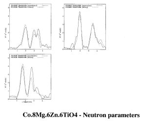
RMC results are calculated using from tables of Co, Al and O contributions from 1.5 to 6 angstroms, and MS contributions of Co-O-Co-Co, Co-O-Al-Co and Co-O-O-Co contributions, with leg-lengths (1.71-2.17)-(4.07-4.68)-(2.13-3.07), for O-O contributions, and (1.71-2.11)-(2.66-3.56)-(1.71-2.11).
.jpg)
.jpg)
.jpg)
.jpg)
Figure 6. Gaussian-broadened histogram of RMC results for: a) Co(Oh), b) Co(Td), c) Ti(Oh), d) Zn(Td).
The results show a marked departure from the accepted crystal structure, with O atoms moving off x,x,x positions. In particular, Ti has a significant contribution at low-r, and on average one essentially non-bonding distance per atom.

RMC output for Co.8Mg.6Zn.6TiO4
Cell Parameters 8.4508 8.4508 8.4508 90.0000 90.0000 90.0000
First scattering atom in MS paths is always: O
***********************************
* CO - Spectrum number 1 *
***********************************
CO Average coordination = 5.47 ( 173 atoms from 1.60 to 2.50)
121.11 double scattering paths with mean length 8.89
Cumulents for all atoms within BOND of CO, + multiplicities
Labels Sub-Shell C1 C2 C3 C4 M
1 CO1(CO)-O8 1.9903 0.0059 0.0000 0.0000 4.00
2 CO4(CO)-O8 2.0701 0.0116 0.0005 0.0001 6.00
Cumulents for sub-shells within RHIGH + multiplicities
1 CO1(CO)-CO1(CO) 2 3.6369 0.0022 0.0000 0.0000 0.70
1 CO1(CO)-CO4(CO) 2 3.5046 0.0061 0.0002 0.0000 3.43
1 CO1(CO)-O8 1 1.9903 0.0059 0.0000 0.0000 4.00
1 CO1(CO)-O8 2 3.5316 0.0145 0.0020 0.0008 12.04
1 CO1(CO)-O8 3 4.4995 0.0089 0.0006 0.0002 11.98
1 CO1(CO)-CO1(MG) 2 3.6712 0.0167 -0.0014 -0.0001 0.74
1 CO1(CO)-CO4(MG) 2 3.5043 0.0148 0.0004 -0.0002 2.46
1 CO1(CO)-CO4(TI) 2 3.4980 0.0053 0.0001 0.0000 6.11
1 CO1(CO)-CO1(ZN) 2 3.6563 0.0070 0.0000 0.0001 2.57
2 CO4(CO)-CO1(CO) 2 3.5046 0.0061 0.0002 0.0000 1.24
2 CO4(CO)-CO4(CO) 1 2.8003 0.0007 0.0000 0.0000 0.13
2 CO4(CO)-CO4(CO) 2 2.9617 0.0056 -0.0001 0.0000 1.57
2 CO4(CO)-CO4(CO) 3 4.9580 0.0016 -0.0001 0.0000 0.16
2 CO4(CO)-O8 1 2.0701 0.0116 0.0005 0.0001 6.00
2 CO4(CO)-O8 2 3.6513 0.0291 0.0015 -0.0004 8.00
2 CO4(CO)-O8 3 4.7561 0.0194 -0.0005 -0.0002 23.05
2 CO4(CO)-CO1(MG) 2 3.4778 0.0196 0.0011 -0.0003 1.16
2 CO4(CO)-CO4(MG) 1 2.7747 0.0013 0.0000 0.0000 0.05
2 CO4(CO)-CO4(MG) 2 3.0524 0.0140 0.0002 -0.0001 1.30
2 CO4(CO)-CO4(MG) 3 4.9566 0.0013 0.0000 0.0000 0.20
2 CO4(CO)-CO4(TI) 1 2.7435 0.0044 -0.0001 0.0000 0.06
2 CO4(CO)-CO4(TI) 2 2.9938 0.0056 0.0002 0.0000 2.90
2 CO4(CO)-CO4(TI) 3 4.9577 0.0017 -0.0001 0.0000 0.20
2 CO4(CO)-CO1(ZN) 2 3.5207 0.0104 0.0001 0.0000 3.60
-------
93.62
Mean bond angles and constituent legs involving bonded atoms, + multiplicities
CO1(CO)-O8-CO4(CO) 119.99( 1.9691 3.5016 2.0774) 3.39( 119.82)
CO1(CO)-O8-CO4(MG) 119.51( 1.9745 3.4884 2.0656) 2.30( 119.40)
CO1(CO)-O8-CO4(TI) 123.14( 2.0055 3.4980 1.9761) 6.11( 122.93)
CO4(CO)-O8-CO1(CO) 119.99( 2.0774 3.5016 1.9691) 1.23( 119.82)
CO4(CO)-O8-CO4(CO) 92.41( 2.0438 2.9497 2.0438) 3.40( 92.38)
CO4(CO)-O8-CO1(MG) 119.58( 2.0671 3.4576 1.9379) 1.08( 119.35)
CO4(CO)-O8-CO4(MG) 93.89( 2.0705 3.0426 2.0942) 2.69( 93.87)
CO4(CO)-O8-CO4(TI) 94.66( 2.0859 2.9909 1.9827) 5.87( 94.60)
CO4(CO)-O8-CO1(ZN) 120.50( 2.0618 3.5111 1.9880) 3.45( 120.21)
Bond Valence= 2.137
***********************************
* TI - Spectrum number 2 *
***********************************
TI Average coordination = 6.00 ( 216 atoms from 1.60 to 2.50)
116.26 double scattering paths with mean length 8.81
Cumulents for all atoms within BOND of TI, + multiplicities
Labels Sub-Shell C1 C2 C3 C4 M
2 CO4(TI)-O8 1.9984 0.0315 0.0055 0.0006 6.00
Cumulents for sub-shells within RHIGH + multiplicities
2 CO4(TI)-CO1(CO) 2 3.4980 0.0053 0.0001 0.0000 1.30
2 CO4(TI)-CO4(CO) 1 2.7435 0.0044 -0.0001 0.0000 0.03
2 CO4(TI)-CO4(CO) 2 2.9938 0.0056 0.0002 0.0000 1.70
2 CO4(TI)-CO4(CO) 3 4.9577 0.0017 -0.0001 0.0000 0.12
2 CO4(TI)-O8 1 1.9984 0.0315 0.0055 0.0006 6.00
2 CO4(TI)-O8 2 3.6758 0.0218 -0.0018 0.0007 8.01
2 CO4(TI)-O8 3 4.7561 0.0185 -0.0008 0.0000 23.09
2 CO4(TI)-CO1(MG) 2 3.5378 0.0138 -0.0007 0.0000 1.06
2 CO4(TI)-CO4(MG) 1 2.8146 0.0000 0.0000 0.0000 0.01
2 CO4(TI)-CO4(MG) 2 2.9483 0.0054 0.0004 0.0000 1.13
2 CO4(TI)-CO4(MG) 3 4.9457 0.0029 -0.0002 0.0000 0.21
2 CO4(TI)-CO4(TI) 1 2.6655 0.0066 0.0000 0.0000 0.36
2 CO4(TI)-CO4(TI) 2 3.0619 0.0102 0.0004 0.0000 2.76
2 CO4(TI)-CO4(TI) 3 4.9438 0.0027 -0.0002 0.0000 0.32
2 CO4(TI)-CO1(ZN) 2 3.5023 0.0127 0.0001 0.0000 3.63
-------
49.75
Mean bond angles and constituent legs involving bonded atoms, + multiplicities
CO4(TI)-O8-CO1(CO) 123.14( 1.9761 3.4980 2.0055) 1.30( 122.93)
CO4(TI)-O8-CO4(CO) 94.66( 1.9827 2.9909 2.0859) 3.45( 94.60)
CO4(TI)-O8-CO1(MG) 123.20( 1.9849 3.5378 2.0452) 1.06( 122.76)
CO4(TI)-O8-CO4(MG) 93.87( 1.9728 2.9466 2.0622) 2.29( 93.79)
CO4(TI)-O8-CO4(TI) 97.23( 2.0261 3.0376 2.0261) 5.94( 97.12)
CO4(TI)-O8-CO1(ZN) 121.94( 2.0094 3.5014 2.0059) 3.62( 121.39)
Bond Valence= 4.035
***********************************
* ZN - Spectrum number 3 *
***********************************
ZN Average coordination = 4.00 ( 130 atoms from 1.60 to 2.50)
141.72 double scattering paths with mean length 9.16
Cumulents for all atoms within BOND of ZN, + multiplicities
Labels Sub-Shell C1 C2 C3 C4 M
1 CO1(ZN)-O8 1.9948 0.0125 0.0017 0.0004 4.00
Cumulents for sub-shells within RHIGH + multiplicities
1 CO1(ZN)-CO1(CO) 2 3.6516 0.0057 -0.0003 0.0000 0.89
1 CO1(ZN)-CO4(CO) 1 3.2774 0.0000 0.0000 0.0000 0.01
1 CO1(ZN)-CO4(CO) 2 3.5213 0.0103 0.0001 0.0000 3.51
1 CO1(ZN)-O8 1 1.9948 0.0125 0.0017 0.0004 4.00
1 CO1(ZN)-O8 2 3.5570 0.0356 0.0062 0.0019 12.41
1 CO1(ZN)-O8 3 4.5268 0.0162 0.0001 0.0002 11.66
1 CO1(ZN)-CO1(MG) 2 3.6664 0.0123 -0.0016 0.0002 0.62
1 CO1(ZN)-CO4(MG) 1 3.2682 0.0001 0.0000 0.0000 0.05
1 CO1(ZN)-CO4(MG) 2 3.5039 0.0187 0.0007 -0.0003 2.37
1 CO1(ZN)-CO4(TI) 1 3.2216 0.0027 -0.0001 0.0000 0.11
1 CO1(ZN)-CO4(TI) 2 3.5069 0.0112 0.0004 0.0000 5.92
1 CO1(ZN)-CO1(ZN) 2 3.6347 0.0075 -0.0001 -0.0001 2.22
-------
43.76
Mean bond angles and constituent legs involving bonded atoms, + multiplicities
CO1(ZN)-O8-CO4(CO) 120.62( 1.9923 3.5207 2.0662) 3.52( 120.33)
CO1(ZN)-O8-CO4(MG) 120.81( 1.9687 3.4973 2.0589) 2.40( 120.52)
CO1(ZN)-O8-CO4(TI) 121.94( 2.0059 3.5014 2.0094) 6.02( 121.39)
Bond Valence= 1.899
Coordinates within cell, 2-4th cumulants, multiplicities, original coordinates
Site(el) PX PY PZ C2X C2Y C2Z C3X C3Y C3Z C4X C4Y C4Z M OX OY OZ
1 CO1(CO) 0.1241 0.1254 0.1254 0.0023 0.0013 0.0021 -0.0001 0.0000 0.0000 0.0000 0.0539 0.0541 1.70( 0.1250 0.1250 0.1250)
2 CO4(CO) 0.5001 0.4998 0.4991 0.0043 0.0043 0.0051 0.0000 0.0000 0.0000 0.0000 -0.6506 -2.5812 4.70( 0.5000 0.5000 0.5000)
3 O8(O ) 0.2610 0.2600 0.2608 0.0098 0.0098 0.0106 0.0002 0.0000 0.0001 0.0002 -0.3716 -0.0862 32.00( 0.2608 0.2608 0.2608)
1 CO1(MG) 0.1208 0.1245 0.1243 0.0098 0.0118 0.0071 0.0001 -0.0004 0.0001 -0.0001 0.1520 0.1400 1.48( 0.1250 0.1250 0.1250)
2 CO4(MG) 0.5001 0.5002 0.4978 0.0096 0.0078 0.0084 0.0002 0.0000 0.0003 0.0000 0.2103 -5.8577 3.30( 0.5000 0.5000 0.5000)
2 CO4(TI) 0.5004 0.5011 0.5010 0.0072 0.0064 0.0065 0.0000 0.0000 0.0001 0.0000 1.6760 1.4720 8.00( 0.5000 0.5000 0.5000)
1 CO1(ZN) 0.1245 0.1245 0.1250 0.0071 0.0073 0.0081 0.0002 -0.0001 0.0002 0.0000 -0.0009 0.0185 4.81( 0.1250 0.1250 0.1250)
-------
56.00
Default Numerical Integral is 4.000
4. Parameters and Related Topics
Parameters are of twenty types :
The first ten groups may be unindexed or have one or two indices :
1. Crystal parameters are unindexed (common parameters), or indexed by phase number - ACELL,BCELL1,CCELL2
2. Atom parameters are indexed by atom numbers - PX1,PT2,OCC3
3. Shell parameters are indexed by shell numbers - N1,T2,X3
4. Unit parameters are indexed by unit number - PANG1,PIV1,UOC2
5. Potential parameters are indexed by atom ic number - MTR8,ALF26 (for O and Fe respectively)
6. Site parameters are indexed by site number - FRA1, FRB2
7. Spectrum parameters are either unindexed (common parameters) or indexed by exafs spectrum number - WEX,EF1,AFAC2
8. Pattern parameters are mostly indexed by pd pattern number - SCALE2, ASYM1, WPD1 ( WPD and BKPOS are unindexed common parameters)
9. Peak profile parameters are either unindexed (common parameters), indexed by pattern number, or indexed by both pattern number and phase - AH, MIXA01, BH12
10. Cluster parameters are indexed by cluster number - XE1, XV2.
There are six groups of unindexed parameters :
11. EXAFS Theory parameters, including those concerned with phaseshift and multiple scattering calculations - LMAX, MINANG 12. PD Theory parameters, - CTHM, WDT, RLIM
13. Control parameters, influencing refinement, output etc. - BOND, SIZE, MAXRAD, STEP29
14. Fourier transform parameters - WP, RMIN, RMAX
15. Surface parameters - ZMIN, DELTAX, SURREL
16. XANES parameters are used only by XANES calculations - XEMIN, XLOUT
There are four additional groups of multiply indexed parameters, where indices are separated by “:” characters :
17. Restrained refinement parameters are indexed by two shell numbers - D3:1,V5:0
18. Bond parameters are index by atom numbers - B253:72
19. Displacement correlation function parameters - C75:4
20. Block parameters - GLa:L2
These parameters may be changed using the command CHANGE (either individually ,or in groups, using a parameter list), or listed using LIST (either individually, in groups, or in pre-defined tables). The majority of the parameters in groups 1-12 may also be refined using REFINE. Many other commands may be used to modify or display parameters (e.g. DISPLAY, PLOT, DRAW, RESET, EXPAND). Parameter lists (e.g. PT[1-3,7-9], A[Ca:L3]), are described in the documentation for the commands CHANGE, LIST and REFINE.
A full list of all the parameters is obtained using INFO PARAM (each individual value is listed using INFO PARAM LONG).
Central atom - each of the clusters represented in the parameter table has one central atom. Cluster 1 has the central atom in shell 0, i.e. has coordinates X0, Y0, Z0 or R0, θ0, φ0. It is often, but not necessarily, at the centre of the coordinate system. The central atom of other clusters may occupy any shell, and is distinguished by a negative cluster number. The central atom is abbreviated by c below.
Absolute and Relative coordinates - the spatial coordinates X, Y, Z, R, θ and φ are all absolute coordinates. If the central atom is not at the origin in these coordinates the theory is determined by the relative coordinates, with the central atom at (0,0,0). It is possible to display, but not to directly change the relative coordinates using LIST RADIAL. Compare thee cordinates given by this command with those given by L SPHL and L CART. To avoid complications it is usually preferable to leave the central atom at absolute position (0,0,0) and to move the ligands. One occasion when this may not be the case is in protein refinements where the main-chain atomic positions are to be retained, but the central atom and ligands such as bicarbonate or hydroxyl are to be moved.
Clusters - the parameter table represents one or more clusters which consists of atoms surrounding crystallographically distinct excited atom sites. A cluster may also be an average over several such sites.
Shell - a shell consists of a set of atoms equidistant from the origin (usually the central atom but see above). Neither the θ nor φ values of the other atoms in the same shell need be the same. If the point symmetry of each central atom is defined, then the coordinates of all the atoms in a shell are defined. If no point symmetry is specified, then for the purpose of theory calculation the coordinates of all te atoms in a shell are assumed to be the same. Many program commands and options are unavailable if the symmetry is undefined.
Unit - a unit is a set of atoms, for example those comprising one ligand, identified by a common, non-zero, unit number. The unit is to allow constrained/restrained refinement, restricted (intra-unit) multiple scattering, and easy addition to, or removal of, ligands from a cluster.
Pivotal atom - the pivotal atom of a unit is the atom about which rotations of the unit are defined. If no pivotal atom is defined, the nearest atom to the centre is assumed. As the nearest atom may change giving unexpected results, it is advisable to set the parameter PIVn to one of the atoms in the unit (i.e. to a shell number) to avoid ambiguity. PIVn then defines the pivotal atom for unit n. In some circumstances, PIVn may be outside the unit (see torsion angles below), it does not then define the pivotal atom. The pivotal atom is abbreviated by p below. The vector c-p is abbreviated by u.
Unit plane - the unit plane is defined by p-a-b, where p is the pivotal atom, a is an atom defined by the unit parameter PLA and b is an atom defined by the unit parameter PLB. The unit plane is defined by the vector n which is a normal to the plane through p. If either p, a or b are undefined ( or equivalent ) then n is taken as a normal to u in the vertical plane. If p is undefined or u is parallel to the z-axis, n is taken as the z-axis.
Principal angle - the principal angle is the angle c-p-a. Its sign is determined by the sign of the z-component of the vector cross-product uX(a-p). If this is zero, the y- or if necessary the -x component is used.
1. Crystal parameters - unindexed or indexed by phase-number
ACELL crystallographic cell dimension a
BCELL crystallographic cell dimension b
CCELL crystallographic cell dimension c
ALPHA crystallographic cell parameter α
BETA crystallographic cell parameter β
GAMMA crystallographic cell parameter γ
PREFA preferred orientation parameter A
PREFB preferred orientation parameter B
DACELL correction to crystallographic cell dimension a
DBCELL correction to crystallographic cell dimension b
DCCELL correction to crystallographic cell dimension c
CLMAX phase dependent MS pathlength
CLMUL phase dependent correction to Debye-Waller factors
These parameters have a common value (applicable to all phases), and indexed values (applicable only to a single phase).
If the spectra and powder patterns are single phase, there is no need to use indexed values. It may then be harder to extend the analysis to multi-phase applications however.
If ACELLn is > 1, then the indexed cell parameters will be used for phase n, otherwise the common values are used. Note that this means you must use either indexed or common parameters for all six cell parameters, and the corresponding correction parameters DACELL etc..
The parameters DACELL etc. are used in multi-pattern fitting Differences in cell parameter may be due to differences in temperature (e.g. ‘Room’ temperatures may vary by 10 degrees or more, beam-heating effects may occur in synchrotron experiments), or to errors in refined values of ACELL etc. (e.g. values from neutron tof experiments are extremely sensitive to sample position).
The preferred orientation parameter used is the sum of the common parameter and the parameter for the phase in question.
The unindexed value of PF is always 1, and is hence ignored. The PF value of the final phase is automatically set to :
1 - the sum of the PF values of other phases
provided this expression is positive or zero.
CLMAXn is used to further restrict the value of multiple scattering pathlength parameter PLMAX for specific phases. PLMAX is a spectrum parameter. The unindexed term has no effect.
CLMULn modifies the Debye-Waller factor for specific phases, when using the DISORDER option BLOCKS. By default it is set to 1. When not equal to 1, then Ada is set to Ga:d1 x CLMULn, where Ga:d1 is the block symbol for atom a in distance group d and spectrum 1. The unindexed term has no effect.
RHIGH determines the maximum cluster size, in Angstroms. The indexed values further restrict the cluster size for specific phases. The value used may be restricted by dimension restrictions, which may be more severe with RMC calculations than with standard theory calculations.
2. Atom parameters - always indexed by phase number
LAB Atom label - an element symbol followed by a 1 or 2 digit number (e.g. CA12)
PT Element used in EXAFS calculations. (‘Pseudo-element’ symbols defined using SITE may also be used).
PI Charge (used only for bond valence evaluation)
SF Symbol for X-ray scattering factor or neutron scattering length (e.g. CA, FE++, or a'pseudo-element' symbol defined using SITE )
PX Fractional coordinate in x-direction
PY Fractional coordinate in y-direction
PZ Fractional coordinate in z-direction
BI Isotropic thermal factor in Å2
PP Phase number associated with the position
PU Unit number associated with the position
Anisotropic temperature factors
The OCC parameters are potentially confusing. They are normally related to Wyckoff number of the site (given by the column labelled 'n(equ)' in LIST POSITIONS. It is not the fractional occupancy. This follows DBW not GSAS usage. Partial occupancy is indicated by reducing the number to a suitable fraction of the Wyckoff number.
These numbers are reset to the Wyckoff numbers if the space group is changed. They may be reset manually using RESET OCC
A ‘pseudo-element’ symbol defined using SITE may be used wherever an element symbol may be used.
The charge PI is used only for bond valence calculation. If a mixed-site symbol is used for PT or SF, then PI is ignored - the bond-valence charge associated with each component of the site is specified when the site is defined (see SITE command documentation). The ionic charge used for exafs potential calculations, is the IONn value where n is the atomic number associated with PT. The ionic charge of an X-ray scattering factor is part of the SF symbol.
The anisotropic temperature factor BI is used, unless the anisotropic term BHH is non-zero for that position. In that case, the sum of the terms in BI and the terms in BHH, BKK ... BLH are used. Symmetry relations within the anisotropic tensor due to the site symmetry must at present be defined manually.
If either BI or non-zero BHH etc. values are less than BIMIN or greater than BIMAX, they will increasing the fit index (soft restraints).
If only one phase is present, PP must be 1 for all positions.
If the unit number PU is non-zero, and is the same value for more than one position, the atoms of the unit will be moved as a rigid body , allowing constrained refinement of the unit.
3. Shell parameters - indexed by shell number
R radial distance of one of the atoms in the shell
A Debye-Waller term 2σ2 (Å2) (or 2 C2 where C2 is the second cumulant of the pair distribution function)
B third cumulant C3 (Å3) x 103
C fourth cumulant C4 (Å4) x 103
D exponent for truncated exponential disorder
UN number of the unit of which the shell is a part, or 0
ANG angle c-p-i for shell i. c = central, p = pivotal atom
TH polar coordinate θ of one of the atoms in the shell
PHI polar coordinate φ of one of the atoms in the shell
X cartesian coordinate x of one of the atoms
Y cartesian coordinate y
Z cartesian coordinate z
ROT rotation about u (unit vector c-p) or VECA-VECB
TWST rotation about n (normal to unit plane)
TILT rotation about nXu (tilt axis)
CLUS cluster to which shell belongs, -ve for an excited atom
FOCC fractional occupation number (single scattering only)
NEXP experiment number associated with the shell
The structural parameters N,T,R,ANG,TH,PHI,X,Y,Z,CLUS and NEXPare normally generated from the position parameters in P, but it is possible to change or refine all of them separately during an exafs-only refinement. The values of structural parameters will be reset using the position parameters, if any of the position parameters are changed, if the space group or point group are changed, if a parameter file is read, if certain RESET or EXTRACT keywords are used, or after an UNDO or RECOVER. They may also be changed following certain errors, or after a DRAW CELL or DISPLAY CELL.
The A parameters may be changed or refined independently if SET DISORDER A is used, otherwise they will be updated from other parameters.
The parameter FOCC is normally 1, and is used to vary the shell occupancy independently of N, and hence of the structural model. It is useful mainly to explore the effect of certain shells on the exafs spectrum, or to determine which shells the exafs spectrum ‘likes’ or ‘dislikes’ during refinement.
The UN parameters allow units to be defined, in order to restrict multiple scattering. They may also be used for constrained refinement during exafs-only refinements.
All the shell parameters may suffer from the effect of the number of shells or order of shells changing when position parameters are refined. For this reason, it is often unwise to directly change or refine shell parameters until the final positional coordinates have been obtained.
N If the point symmetry of the cluster is defined, the occupation numbers must be an integer number consistent with the symmetry position occupied. This may sometimes mean that a shell of atoms must be split into two - as for HCP structures where c/a is exactly (8/3)1/2.
T The atom type is stored as a number, which is the same as that used in reading phaseshift files and in indexing phaseshift variables, including the ATOMn variables, where the index n corresponds to the value of T. If the ATOM variables are defined, then T may be assigned an element symbol instead of a number.
R When the central atom of the cluster is at the centre of the coordinate system, the R values of all the atoms in a shell are there same. This is not the case, however, when the central atom has other coordinates.
ROT ROT defines a rotation about an axis, but there is no absolute reference for the rotation, so only the change in its value is significant. For this reason it is often simpler to enter commands such as C ROT13 ROT13+90. The axis used is determined by the parameters VECA and VECB which determine two points defining the rotation vector. VECA is always a shell number ( 0 for central atom of cluster 1). VECB may be a positive shell number, negative, or zero :
VECB > 0 the second point is shell VECA ( not shell 0)
VECB = 0 the second point is the pivotal atom for the unit to which the shell belongs ( the unit must be defined).
VECB < 0VECB is a code defining a direction relative to VECA. These codes are -1 for <100>, -2 for <010>, -3 for <001>, and -4 for <111>. What -5 does is a complete mystery.
Note that if, as is often the case, the central atom in shell 0 is required, this must be specified as VECA not VECB.
CLUS This parameter determines which cluster the shell belongs to and whether the shell is an excited atom or not. An excited atom is signified by a negative value.
LINK If two excited atoms are in close proximity, such as for Fe atoms in cubane, it would be normal to link one cluster with the other. This is achieved by setting the LINK parameter for a shell in one cluster to a shell in another, and defining an offset vector for the second cluster. This is normally done by means of the command GENERATE, but (in recent versions) LINKS may be inspected or changed manually.
Special rules apply to to shell parameters during constrained refinements, i.e. with CONSTRAINTS ON (see the constrained refinement section of chapter 2).
1. Movement of the pivotal atom, either along a vector passing through the central atom (X, Y, Z or R), or by means a rotation about an axis passing through the central atom (TH, PHI, ROT, TWST and TILT). This occurs when the shell of a pivotal atom is changed. e.g., if the pivotal atom for unit 1 is in shell 7, then a command might be C R7 2.2 or C R[PIV1] 2.2.
The rules governing motion in this case are :
R motion is along the vector c-p so that the pivotal atom has the new R value requested.
TH the unit is rotated about an axis through c and normal both to u and the z-axis, so that the new value of theta for the pivotal atom is achieved.
PHIthe unit is rotated about and axis though c and parallel to the z-axis so that the pivotal atom has the new coordinate requested.
X the unit is translated along a vector through c parallel to the x-axis.
Y translation parallel to the y-axis.
Z translation parallel to the z-axis.
ANG as the c-p-p angle is undefined (0) this is not a valid option.
ROT the unit is rotated about the vector defined by VECA and VECB. The user must ensure that VECA refers to the central atom and VECB is neither 0 nor the pivotal atom.
TILT the unit is rotated about the tilt axis nXu by the change in value.
TWST the unit is rotated about n the normal to the unit plane.
All these type A motions are straightforward if the central atom is at the centre of the coordinate system (0,0,0). If this is not the case, motion is more complex as the parameter values to be satisfied are the absolute values not the values relative to the central atom. Under these circumstances, some values or PHI may be unobtainable, and the program does not allow TH to be changed at all. None of these type A motions will effect the single scattering or intra-unit multiple scattering EXAFS except for R, provided POLARISATION is set to off.
2. Movement of one of the atoms other than the central or pivotal atom. In every case this involves a rotation about an axis passing through the pivotal atom, while the position of the pivotal atom itself is unchanged. This occurs
When any shell variables associated with the unit other than those of the pivotal or central atoms are changed. E.g. C R7 2.2 or C R[PLA1] 2.2. Note that C PANG1 235 is exactly equivalent to C ANT[PIV1] 235.
The rules governing motion in this case are :
R The unit is rotated about the tilt axis uXn
TH the unit is rotated about the tilt axis uXn
PHI the unit is rotated about n the normal to th unit plane
X,Y the unit is rotated about n
Z the unit is rotated about the tilt axis uXn
ANG the unit is rotated about uX(s-p), where s is the vector defining the shell in question
ROT the unit is rotated the axis defined by VECA and VECB
TWST the unit is rotated about n
TILT the unit is rotated about the tilt axis uXn
4. Unit parameters - indexed by unit number
PLA atom a defining the unit plane, and the principal angle
PLB atom b defining the unit plane
TORA torsion angle ψ (N-CA-CB-CG)
TORB torsion angle ϖ (CA-CB-CG-CD)
TORC torsion angle at centre (c-p-a-b)
UOC unit occupancy - changes N for all atoms in the unit
All the parameters above can be changed using the command CHANGE, or can be refined using REFINE as well as being read from files. A number of other unit variables can only be modified by reading from the ligand database, or from a Brookhaven (.pdb) file or by changing them interactively using PLOT UNIT. These are :
NTORA[1-4] the atoms defining torsion angle A
NTORB[1-4] the atoms defining torsion angle B
RESNAME the name of the ligand ( residue in .PDB files)
5. Potential parameters - indexed by ATOMIC NUMBER, or in two cases by CLUSTER NUMBER., or unindexed
ALF exchange term for X-α ground state exchange
CMAG Correction to Madelung potential (Rydberg units)
NGRID number of points in grid used for potential calculations
PC Number of neighbours, which also determines the structure
V0 global interstitial potential value for potential calculation (eV)
FE0 global Fermi energy value for potential calculation (eV)
RHO0 global charge density value for potential calculation (4/3πr2 x e/(bohr rad)3)
See also the spectrum parameters CW which are used in calculating phaseshifts from the potentials and the theory parameter NGRID which determines the number of points in the logarithmic grid used in potential calculations.
MTRs have program default values which can be listed using INFO MTR [-1,0,1], where the option number designates anion, neutral atom or cation values). They may be changed or refined, provided SET COMMON NONE (the default option) is selected. Default values may be restored using RESET MTR. If the COMMON options V, RHO, EFERMI or ION are selected, then the MTRn are adjusted so as to achieve the current value of V0, RHO0, FE0 or IONn.
ION is usually 0, as ionic phaseshifts, at least for binary compounds, produce fits which differ from neutral atom phaseshifts little except in the refined value of EF. Moreover, only a few anion charge densities are available (O-, F- ..), and these are not entirely reliable.
6. Site parameters used for adjusting the occupancy of mixed sites
FRAi Fraction of component A in site i
FRBi Fraction of component B in site i
FRCi Fraction of component C in site I
FRDi Fraction of component D in site i
SITEBi Component B in site i
SITECi Component C in site i
See command SITE for details
7. Spectrum parameters (EXAFS)
Most of these variables are unindexed, but some, such as EF, AFAC, EMIN, EMAX have a spectrum index. For these variables, as well as a common variable, which applies to all spectra, there are individual variables which apply to only one (some of these only apply to most recent versions of the program). These are indexed by spectrum number, as used in READ EXP. Variables of this type are indicated by an optional index below. e.g. EF(i).
EF(i) edge position (fermi energy), relative to calculated vacuum zero
VPI(i) energy-independent correction imaginary potential
AFAC(i) amplitude reduction due to many-electron processes etc.
BETHi beam direction - theta value, for spectrum i
BEPHIi beam direction - phi value, for spectrum i
BEWi polarisation azimuth, for experimental spectrum i
CW(i) the effective core-hole width, in eV. Theoretical values used if -1
DE(i) spectrum specific correction to E0, used in whole-spectrum fitting
EMIN(i) minimum energy for EXAFS theory calculations
EMAX(i) maximum energy for EXAFS theory calculations
KMIN(i) minimum wave vector for EXAFS theory
KMAX(i) maximum wave vector for EXAFS theory
PLMIN(i) minimum pathlength for multiple scattering paths
PLMAX(i) maximum pathlength for multiple scattering paths
coefficients of pre-edge correction factor for whole-spectrum fitting (not currently implemented)
coefficients of polynomial correction factor for whole-spectrum fitting
WB(i) weighting for Bond valence sum component of the fit-index
WEX(i) weighting for EXAFS component of the fit-index
In some instances it may be useful to combine common and individual variables - e.g., AFAC may be the same for all but one of the spectra. The rules for combining variables, in the case of spectrum i is as follows :
AFAC The program uses AFAC*AFACi
EMIN The program uses MAX(EMIN,EMINi)
EMAX The program uses MIN(EMAX,EMAXi)
KMIN The program uses MAX(KMIN,KMINi)
KMAX The program uses MIN(KMAX,KMAXi)
CW The program uses CW unless CW=-1, when it will use CWi unless that is -1, for spectrum i. If both terms are -1, program default values are used
WEX The program uses WEX*WEXi
WB The program uses WB*WBi
BETH There is no BETH - it uses BETHi (similarly with BEPHI, BEW)
The common variables may also be written, for example, EF0. This can be useful in resetting variables. e.g.
C AFAC[0-3] 1
Beam Parameters
Beam parameters are used in polarised (single crystal or surface) EXAFS to describe the orientation of the beam in terms of the axial system used to describe the crystal. There are three sets of beam parameters, used to describe each of the experimental files which have been read in (e.g., BETH1, BETH2, BETH3). The beam orientation is given by BETH1 and BEPHI1 etc., the polarisation direction by BEW1. The default settings are for the polarisation e vector parallel to x, y and z respectively. The parameter values and the corresponding e vector directions are shown below.
l spars
Spectrum 1 Spectrum 2 Spectrum 3
BETH1 = 0.000 BETH2 = 0.000 BETH3 = 90.000
BEPHI1= 0.000 BEPHI2= 0.000 BEPHI3= 0.000
BEW1 = 90.000 BEW2 = 0.000 BEW3 = 90.000
EX1 = 1.000 EX2 = 0.000 EX3 = 0.000
EY1 = 0.000 EY2 = -1.000 EY3 = 0.000
EZ1 = 0.000 EZ2 = 0.000 EZ3 = -1.000
ETH1 = 90.000 ETH2 = 90.000 ETH3 = 180.000
EPHI1 = 0.000 EPHI2 = 270.000 EPHI3 = 0.000
8. Pattern parameters (powder diffraction) - unindexed or indexed by pattern number
BACK0 background parameter - zero'th order
BACK1 background parameter - 1st order
BACK2 background parameter
BACK3 background parameter
.......
BACK17 background parameter
CTHM Monochromator coefficient in polarisation correction
BKPOS(i) Origin of background polynomial
DIFA(i) coefficient of d^2 in time-of-flight definition
DIFC(i) coefficient of d in time-of-flight definition
DTERM(i) Absorption correction coefficient
OFFSET(i) Offset of sample from its ideal position
SCALE(i) scale - defined as 10^6 * DBW quantity
THETA(i) Neutron detector position
WPD(i) weighting for PD component of the fit-index
ZER(i) Zero error in the monochromator calibration
9. Peak profile parameters (powder diffraction)
AH(ij) peak width parameter, coefficient of tan2θ (independent term for tof)
BH(ij) peak width parameter, coefficient of tanθ (coefficient of d for tof)
CH(ij) constant peak width parameter (cofficeient of d2 for tof)
XH(ij) Lorentzan peak width parameter for TCH-pV
YH(ij) Lorentzan peak width parameter for TCH-pV
ZH(ij) peak width parameter, coefficient of 1/cos2θ
DECA independent term in exponential rise coefficient
DECB dependent term in exponential rise coefficient
DECC independent term in exponential fall coefficient
DECD dependent term in exponential fall coefficient
KAPPA exponent in tof profiles
GAMA(ij) Independent Lorentzian peak width parameter
GAMB(ij) Lorentzian peak width parameter, coefficient of d
GAMC(ij) Lorentzian peak width parameter, coefficient of d2
GAMD(ij) Lorentzian peak width parameter, coefficient of d cosθ
GAME(ij) Lorentzian peak width parameter, coefficient of d2 cosθ
MIXA(ij) constant pV mixing parameter
MIXB(ij) pV mixing parameter, coefficient of 2θ
MIXC(ij) constant pV mixing parameter, coefficient of (2θ2)
Peak width and peak profile parameter usage depends on the profile function.
Most functions depend on a Gaussian and/or Lorentzian half-width given by :
![]()
![]()
except for the Modified TCH-Pv function where :
![]()
or in the time-of-flight case by
![]()
and
![]()
For a pseudo-Voigt function, the profile is defined as :
and therefore involves 6 parameters - AH, BH, CH, ZH, MIXA, MIXB (ZH invariably 0)
The modified Lorentzian functions involve only L, and hence 4 parameters (AH, BH, CH, ZH)
The Pearson function is given by :
and thus has 8 parameters, AH, BH, CH, ZH, MIXA, MIXB, MIXC
The Modified TCH pseudo Voigt function depends only on G and L (second definition), and so has 6 parameters, AH, BH, CH, XH, YH, ZH
The time-of-flight functions are :
TOF2
which depends on the terms :

There are therefore 12 parameters, AH, BH, CH, GAMA, GAMB, GAMC, GAMD, GAME, DECA, DECB, DECC and KAPPA
TOF3 :

There are therefore 12 parameters, AH, BH, CH, GAMA, GAMB, GAMC, GAMD, GAME, DECA, DECB, DECC and KAPPA
10. Cluster parameters
XE Cluster-specific correction to EF
XV Cluster-specific correction to VPI
Cluster numbers CLUSn for shell n are normally generated automatically when the radial coordinates are produced. These parameters are used when the same phaseshifts are used for all similar atoms, but where the ionic charge on the atoms are different (e.g.Co2+ and Co3+). There is no need to use these parameters if CALC POT X is used (phaseshifts are then cluster dependent). XV and VPI should normally be avoided. These parameters should be set to zero when using RMC - either when generating tables or doing actual calculations.
AOFF enrgy zero for atomic correction 0
ATMAX maximum number of different atoms in a MS path
CLE coefficient of linear expansion - if ne 0, used to calculate T-dependent C3 in anharmonic oscillator model
DLMAX maximum angular momentum for double-scattering theory
DPXHH off-centre displacementin x-direction for heavy atom-heavy atom pairs
DPXHL off-centre displacementin x-direction for heavy atom-light atom pairs
DPXLH off-centre displacementin x-direction for light atom-heavy atom pairs
DPXLL off-centre displacementin x-direction for light atom-light atom pairs
DPYHH off-centre displacementin y-direction for heavy atom-heavy atom pairs
DPYHL off-centre displacementin y-direction for heavy atom-light atom pairs
DPYLH off-centre displacementin y-direction for light atom-heavy atom pairs
DPYLL off-centre displacementin y-direction for light atom-light atom pairs
DPZHH off-centre displacementin z-direction for heavy atom-heavy atom pairs
DPZHL off-centre displacementin z-direction for heavy atom-light atom pairs
DPZLH off-centre displacementin z-direction for light atom-heavy atom pairs
DPZLL off-centre displacementin z-direction for light atom-light atom pairs
DTEMP Debye temperature, used in generating thermal parameters by Debye theory
E0 absolute edge position - for whole-spectrum fitting only
EOFF fitting parameter defining the independent variables origin in the whole-spectrum polynomial correction
POLM mass term in expression for DCF
POL0 constant term in expression for DCF
POL1 r-dependent term in expression for DCF
POL2 r2-dependent term in expression for DCF
HEAVY defines heavy atom for off site displacements
LIGHT defines light atom for off site displacements
LMAX maximum angular momentum for single scattering theory
LOP partial ordering parameter
DPP displacement parallel to M-M vector
DPN displacement normal to M-O-M plane
MBOND upper limit in r for mixed-mode MS
MINANG minimum angle for multiple scattering paths
MINDIST minimum distance for inter-atomic paths in multiple scattering paths
MINMAG minimum magnitude in principal path selection
NGRID number of points in grid used for potential calculations
NPOST number of polynomial terms
NS the number of shells used for calculations
NSPEC number of spectra actively involved in EXAFS calculations
NUMAX matrix size in seperable approximations. 0 for small atom, 2 for R+A full matrix
OMIN minimum order of scattering for theory calculations
OMAX maximum order of scattering for theory calculations
QM mass-coefficient for parameterised DW factors
QMS mass2-coefficient for parameterised DW factors
QR r-coefficient for parameterised DW factors
QRS r2-coefficient for parameterised DW factors
QT constant term for parameterised DW factors
QS coefficient for parameterised DW factors
PE0 energy threshhold for linear correction to atomic absorption
PE1 linear coefficient for correction to atomic absorption
TEMP temperature (K) - used in calculating edge-width (whole-spectrum fitting) and C3 (if CLE ne 0)
TLMAX maximum angular momentum for triple-scattering theory
Multiple Scattering Parameters
A number of parameters apply only to MS. DLMAX and TLMAX determine the number of angular momentum terms for double and triple scattering respectively. Although the number of terms required is usually less than for single scattering, the maximum values of 12 and 9 rather than the default values of 6 and 5 will be required for heavy atom scatterers.
Several parameters restrict the number of paths that are calculated. These parameters can also be used to isolate contributions using EXTRACT if a full set of paths have been previously calculated.
ATMAX determines the maximum number of scattering atoms in a path - default is 2. 3, 4 or 5 may be selected at high computational expense.
MINANG is the minimum angle - scattering within a triplet of atoms, or a quadruplet derived from it, will not be calculated unless one of the bond angles exceeds this value.
MINDIST determines the minimum permitted distance in any MS path. When site vacancies are being used it can be used to avoid including a disordered site twice in the same path. It also determines the minimum acceptable distance for RMC simulations. In this context it acts as a hard constraint if MW=0, or a soft restraint if MW is positive.
MINDISL determines the minimum permitted distance between two atoms of similar type in RMC calculations. Must therefore be longer than MINDIST.
MINMAG determines a cut-off below which previously calculated paths will be ignored. Default is 0. This should be used with great care. If one of the above parameters is changed, or any bond length changes by more than a few percent, the path indices will change, causing the wrong paths to be omitted. Path indices may be inspected using EXTRACT. A safe way to use this, is to set MINMAG to 0, calculate a spectrum with small atom or low DLMAX and TLMAX, set MINMAG to a sensible cut-off, and recalculate the spectrum using a higher angular momentum.
OMIN is the minimum order - default is 1
OMAX is the maximum order - default 3, maximum 5 - use of a higher order will considerably slow down the calculations.
PLMIN is the minimum path length ( usually 0 )
PLMAX is the maximum path length (default is 10)
The command LIST MSPARS will give the current values of most multiple scattering parameters.
When using the SMALL_ATOM option (SET THEORY SMALL_ATOM), the precision may be selected using NUMAX, which determines the size of the scattering matrix. 0 uses the approximation of Gurman (1988), 1 and 2 use the Rehr and Albers (1990) method, where the value of NUMAX determines the matrix size.
12. Powder diffraction theory parameters
RLIM maximum d-spacing for which asymmetry corrections apply
NBACK number of powder diffraction background terms
TOLER tolerance factor in complex exponential integral evaluation
TRANSP transparancy correction coefficient
WDT peak width control (multiple of FWHM)
BISO constant isotropic temperature factor. This is used mainly with RMC calculations, where EXAFS and PD DW factors are systematically different, due to errors associated with small partical size etc. It should normally be 0.
RELAX relaxation factor during minimisation
The EXAFS theory parameter DTEMP also applies to PD. A number of control parameters relate to PD calculations. Most crystal, atom, pattern, peak-shape and phase parameters effect PD calculations.
BANK powder diffraction bank number use d in reading GSAS files
BOND controls bond distances with DRAW and DISPLAY, and bond valence calculations
D1A parameter A for use with CHANGE D1
D1B parameter B for use with CHANGE D1
D2A parameter A for use with CHANGE D2
D2B parameter B for use with CHANGE D2
DWMIN minimum reasonable value of A
DWMAX maximum reasonable value of A
EPS Controls the minimisation procedure, refinement terminates when all calues change by less than EPS.
OUTPUT determines the output level
DFAC Relates maximum to initial step size in REFINE
NIND number of independent points in χ2 calculation
NPARS number of refined parameters used in χ2 calculation
NPOS number of atomic positions in all phases
NSITES number of SITES that have been defined
SIZE atom size in plots (% of MTR)
SPAR11 suppress pi-shift if 99 - should normally be 97
SNOISE amplitude of noise component of theory
TMIN minimum 2θ value for XRD plots
TMAX maximum 2θ value for XRD plots
VX x-coordinate of viewing position for 3D plots
VY y-coordinate of viewing position for 3D plots
VZ z-coordinate of viewing position for 3D plots
WANG weighting for angle restraint component of the fit-index
WD weighting for distance restraint component of the fit-index
WNOISE k-weighting of noise component of theory
YMIN y-axis minimum for plots (for GSET RANGE YMIN/YMAX)
YMAX y-axis maximum
For additional weighting terms used in calculating the fit index see spectrum parameter WEX and pattern parameter WPD.
14. Fourier transform parameters
RMIN minimum distance for Fourier transforms
RMAX maximum distance for Fourier transforms
WP Fourier transform window parameter
The Fourier transform calculation is also influenced by the FTSET options, which include the way the k- and r-space spectra are weighted.
15. Surface parameters - NOT CURRENTLY IMPLEMENTED
ZMIN minimum depth of surface layer
ZMAX maximum depth of surface layer
DELTAX substrate displacement in x-direction
DELTAY substrate displacement in y-direction
DELTAZ substrate displacement in z-direction
SURROT surface rotation - rotation of top layer of substrate
SURREL surface relaxation - increase in top layer spacing relative to bulk
The following parameters are, like phaseshifts, indexed by atomic number, but are involved in changing the structure, not the phaseshifts
SDXi Displacement in x-direction for atoms of type i with Z between ZMIN and ZMAX
SDYi Displacement in y-direction for atoms of type i with Z between ZMIN and ZMAX
SDZi Displacement in z-direction for atoms of type i with Z between ZMIN and ZMAX
Surface displacement parameters
The surface displacement parameters DELTAX, DELTAY, DELTAZ and those indexed by atoms type, - SDX, SDY, and SDZ, are used for correlated movement of surface atoms. They are specific to surfaces, are indifferent to the status of the CONSTRAINTS option and do not require the use of units.
DELTAX etc. will move all atoms other than those in the z >=0 adsorbate layer in the required direction (in the cartesian rather than the crystallographic cell). For example DELTAX or DELTAY will simulate movement of the adsorbate off a high symmetry site, while DELTAZ will alter the adsorbate-substrate distance. Note that because all atoms, including those in special positions, are moved, the use of these parameters is highly subject to the point symmetry of the cluster. Movement of DELTAZ is not permitted in point groups with a centre, a horizontal mirror plane, a horizontal diad or cubic symmetry. However, as these are improbably in a surface simulation these restrictions should not prove a problem. DELTAX and DELTAY however are incompatible with a principal axis higher than 1, and are effectively restricted to use with ci and cx. cx is a specially defined point group symbol representing cσ in an alternative orientation with the mirror plane parallel to x. As DELTAX etc. have no absolute origin as a reference point, only changes in its value are relevant, so atoms are moved by the difference between the new and old values.
SDX etc. operate in a manner analogous to DELTAX etc.. The differences are that SDX only moves atoms in the top substrate layer, or surface layer, and is indexed by atom type, so that only certain atoms are moved. The surface layer is defined to mean any atom with a z-coordinate between ZMIN and ZMAX angstroms. If the atoms to be moved are in a general position then there are no symmetry restrictions on which movements are allowed. If atoms are in a special position with respect to a point symmetry operator, such as lying on the principal axis, then symmetry restrictions will apply. These will not be checked when the change is made, as with DELTAX, and will result in errors the next time the coordinates of all the atoms are expanded using the point group symmetry. If it is necessary to distinguish crystallographically distinct sites occupied by the same atom type, it will be necessary to duplicate phaseshifts, and assign two different atom types to the same element.
The action resulting from such movements will clearly depend on which of the set of symmetry related atoms are given in the table of shell parameters. With DELTAX the symmetry rules ensured that all the atoms were translated in the same direction. With SDX however, the action of vertical mirror planes will cause contrary motion of individual atoms and non-unitary principal axes will cause rotations. Indeed, the principal use of these variables is to simulate surface reconstructions which involve rotations of atoms, in contrary directions for adjacent adsorbate sites. The effect of the symmetry operator will be different depending on which atom in a shell has been selected for each shell ( they will simulate the effect of different crystallographic space groups). In general, only one of the possible choices is correct, and this will not be the case which is usually selected. An example of a parameter table ( for reconstructed p4g N on Ni(100) is given below.
l car
E0 = 3.000 VPI = -4.000 AFAC= 0.800 EMIN= 3.000 EMAX=3000.000
RMIN= 0.100 RMAX= 10.000 WIND= 2.000 WP = 0.100 NS = 10.000
Shell 1 N1 = 4.000 T1 = 28(NI) X1 = 2.400 Y1 = 0.000 Z1 = -1.000
Shell 2 N2 = 4.000 T2 = 28(NI) X2 = -2.400 Y2 = 4.800 Z2 = -1.000
Shell 3 N3 = 4.000 T3 = 28(NI) X3 = -2.400 Y3 = -4.800 Z3 = -1.000
Shell 4 N4 = 4.000 T4 = 28(NI) X4 = -7.200 Y4 = 0.000 Z4 = -1.000
Shell 5 N5 = 4.000 T5 = 8 (O ) X5 = 0.000 Y5 = 4.800 Z5 = 0.000
Shell 6 N6 = 4.000 T6 = 8 (O ) X6 = 4.800 Y6 = 4.800 Z6 = 0.000
Shell 7 N7 = 1.000 T7 = 28(NI) X7 = 0.000 Y7 = 0.000 Z7 = -2.200
Shell 8 N8 = 4.000 T8 = 28(NI) X8 = 4.800 Y8 = 0.000 Z8 = -2.200
Shell 9 N9 = 4.000 T9 = 28(NI) X9 = 2.400 Y9 = 2.400 Z9 = -2.200
Shell 10 N10= 4.000 T10= 28(NI) X10 = 4.800 Y10 = 4.800 Z10 = -2.200
l frac
Cell parameters: 9.6000 9.6000 1.0000
Shell X Y Z
0 O 0 0.0000 0 0.0000 0 0.0000
1 NI 0 0.2500 0 0.0000 -1 0.0000
2 NI -1 0.7500 0 0.5000 -1 0.0000
3 NI -1 0.7500 -1 0.5000 -1 0.0000
4 NI -1 0.2500 0 0.0000 -1 0.0000
5 O 0 0.0000 0 0.5000 0 0.0000
6 O 0 0.5000 0 0.5000 0 0.0000
7 NI 0 0.0000 0 0.0000 -3 0.8000
8 NI 0 0.5000 0 0.0000 -3 0.8000
9 NI 0 0.2500 0 0.2500 -3 0.8000
10 NI 0 0.5000 0 0.5000 -3 0.8000
c sdy2 .02
l car
EF = 3.000 VPI = -4.000 AFAC= 0.800 EMIN= 3.000 EMAX=3000.000
RMIN= 0.100 RMAX= 10.000 WIND= 2.000 WP = 0.100 NS = 10.000
Shell 1 N1 = 4.000 T1 = 28(NI) X1 = 2.400 Y1 = 0.192 Z1 = -1.000
Shell 2 N2 = 4.000 T2 = 28(NI) X2 = -2.400 Y2 = 4.992 Z2 = -1.000
Shell 3 N3 = 4.000 T3 = 28(NI) X3 = -2.400 Y3 = -4.608 Z3 = -1.000
Shell 4 N4 = 4.000 T4 = 28(NI) X4 = -7.200 Y4 = 0.192 Z4 = -1.000
Shell 5 N5 = 4.000 T5 = 8 (O ) X5 = 0.000 Y5 = 4.800 Z5 = 0.000
Shell 6 N6 = 4.000 T6 = 8 (O ) X6 = 4.800 Y6 = 4.800 Z6 = 0.000
Shell 7 N7 = 1.000 T7 = 28(NI) X7 = 0.000 Y7 = 0.000 Z7 = -2.200
Shell 8 N8 = 4.000 T8 = 28(NI) X8 = 4.800 Y8 = 0.000 Z8 = -2.200
Shell 9 N9 = 4.000 T9 = 28(NI) X9 = 2.400 Y9 = 2.400 Z9 = -2.200
Shell 10 N10 = 4.000 T10= 28(NI) X10 = 4.800 Y10 = 4.800 Z10 = -2.200
l frac
Cell parameters: 9.6000 9.6000 1.0000
Shell X Y Z
0 O 0 0.0000 0 0.0000 0 0.0000
1 NI 0 0.2500 0 0.0200 -1 0.0000
2 NI -1 0.7500 0 0.5200 -1 0.0000
3 NI -1 0.7500 -1 0.5200 -1 0.0000
4 NI -1 0.2500 0 0.0200 -1 0.0000
5 O 0 0.0000 0 0.5000 0 0.0000
6 O 0 0.5000 0 0.5000 0 0.0000
7 NI 0 0.0000 0 0.0000 -3 0.8000
8 NI 0 0.5000 0 0.0000 -3 0.8000
9 NI 0 0.2500 0 0.2500 -3 0.8000
10 NI 0 0.5000 0 0.5000 -3 0.8000
The surface relaxation parameter SURREL
SURREL alters the surface relaxation - that is, the distance between the top two substrate layers of a surface relative to the bulk interlayer spacing. The default value is 1. As with SDX etc. the surface layer is defined as that between ZMIN and ZMAX. When changing SURREL care should be taken to ensure that as a result of the change, atoms within the surface layer do not move out of it, and that atoms outside the surface layer do not move into it.
XMIN minimum energy for XANES theory calculations
XMAX maximum energy for XANES theory calculations
XNP number of points in XANES calculations
XLMAX maximum angular momentum for XANES calculations
XLOUT maximum angular momentum for single centre expansion
XOPT determines treatment of central atom phase.
17. Restrained refinement parameters
Dn:m ideal distance from atom n to m
Wn:m weighting forl distance Dn:m
An:m ideal angle n-0-m
Vn:m weighting for angle An:m
WD weighting for distance restraint component of the fit-index
WA weighting for angle restraint component of the fit-index
Ba:b include bond a-b in DRAW output, irrespective of the value of BOND
19. Displacement correlation function parameters
Ca:b DCF for atom pair 1-b
Ga:b Value of A to be used atom a in block b. If further indexed by a number, will relate specifically to that spectrum.
E.g. GAl:I2 - will be used to set the A values for Al atoms at intermediate distance for spectrum number 2.
Four control parameters are used in connection with the block method for treating EXAFS Debye-Waller factors. They are repeated here for convenience.
VSHORT Defines the upper limit of the vshort block (includes all shells between 0 and VSHORT)
SHORT Defines the upper limit of the short block (includes all shells between VSHORT and SHORT)
LONG Defines the upper limit of the intermediate block (includes all shells between SHORT and LONG)
XLONG Defines the upper limit of the long block (includes all shells between SHORT and LONG)
Shells between XLONG and infinity constitute the xlong block.
The G symbols provide an easier way of handling the list form of A symbols when using the DISORDER BLOCKS option.
So C A[O:S1] .01 is the same as C GO:S1 .01, and REFINE BLOCKS will use G symbols rather than A’s.
It is not possible to use rules to define values of G symbols. This effect may however be achieved using A symbols. A special option RULE AUTOGENERATE is available to help set up rules, which may be very complicated. For example, it is normally necessary to ensure that A[Cu:L1] is the same as A[Au:L2] if spectrum 1 is Au and 2 is Cu.
Rules set for symbols not indexed by spectrum number, will not apply if symbols which are indexed by spectrum number are used.
ALIAS is used to define commands.
Syntax: ALIAS alias_name [DEL]
ALIAS [LIST]
ALIAS DELETE [n]
Abbreviations: AL
This command allows users to define their own commands or abbreviations. For example :
ALIAS TEMPCOM
results in the prompt :
Enter definition of TEMPCOM :
You can then type in any command or list of commands e.g. :
gset dev 2;gset plotter ps_file
and for the rest of the session TEMPCOM will result in the execution of the list of commands.
If LIST is specified or else the command is entered without a keyword, then ALIAS lists the current aliases.
The number of aliases which may be defined is displayed using LIST DIMENSION. An alias may be up to 80 characters long. If the maximum number of aliases are already defined, the last n may be deleted using ALIAS DELETE n. If n is unspecified, the default is 1. DELETE may not be abbreviated, so that alias names such as DEL are allowed.
A specific alias may be deleted using :
ALIAS alias_name DEL
Aliases containing special characters such as *, % and ! should be enclosed in quotes :
ALIAS LL;'*ls -l'
Once defined, an alias may be used whenever a command name may be used.
An alias name must not conflict with an existing command or abbreviation. For example :
ALIAS R;C R1 2
Will have no effect, as R will always be interpreted as READ, for which it is a permitted abbreviation.
CALC is used to calculate potentials and phaseshifts.
Syntax: CALC POTENTIALS [n/el]
CALC PHASESHIFTS [n/el]
Abbreviations: CA PO/PH
Option: atom number n or element el
If the number n is defined then the calculation is performed for potentials or phaseshifts previously specified as pertaining to spectrum n. If element el is specified (with or without n), only potentials relating to that element is calculated. An excited atom should be specified as el* (e.g. CU*). These options are only valid after potentials or phaseshifts have been calculated for the complete set of atoms (CALC POT or CALC PHASE).
e.g. CA POT
Will calculate potentials for: Central (excited) atoms for each spectrum (up to the current value of NSPEC)
All atoms in the POSITIONS table
All atoms in the SHELLS table
All atoms which are components of MIXED SITES
The potentials or phaseshifts are calculated using the approximations and methods outlined in the theory section.
Options which apply to potential calculations include those available through SET GROUND_STATE, SET EXCHANGE, SET COMMON and SET SHARE_PHASE (see the command documentation for SET).
Options which apply to phaseshift calculations include those available through SET QUINN, SET RELCOR (see the command documentation on SET).
Variables which apply to potential calculations for element n, include PCn, MTRn, IONn, and CMAGn. Other variables affecting potential calculations, when using COMMON options, include V0, FE0 and RHO0.
Phaseshift calculations for experiment i use the core-hole width parameters CWi or the common core-hole width parameter CW.
CALC issues many prompts whose significance are described in the sections Calculating Potentials and Calculating Phaseshifts of the Program Guide (chapter 2). An example potential calculation is described in the examples section.
For Whole-spectrum fitting - using SET ATOMIC_ABS ON, slightly different rules apply in the case of CALC PHASE. The atomic transition rate will be calculated by default for each central atom, using an entirely real potential, as the treatment of inelastic effects is inappropriate for calculation of dipole transition rates. Temperature dependent broadening due to the distribution of electrons in the valence band, and lifetime/experimental broadening is included when the theoretical spectrum is calculated.
CHANGE is used to alter the values of the parameters described in section 4.
Syntax: CHANGE variable_name new_value
Abbreviations: CH or C
Notes:
The effect is to change the value of variable_name to new_value.
Variable_name may be one of :
a) A parameter name, R1, EMIN etc. ( see the parameters section for a full list). Note that the program will not allow some parameters to be changed to values outside a specified range. Some parameters ( EMIN, EMAX, EF, KMIN, KMAX ) are interconnected and may change if you change the others (The relationship between KMIN and EMIN depends not only on EF, but also on the energy dependent self-energy, and may change when the theory is updated). New_value is usually a number, but in the case of parameters such as Tn, new_value may be either an atomic number or chemical symbol :
C T1 CU is equivalent to C T1 29
Parameters D1A, D1B, D2A and D2B are CHANGEd to the name of another parameter ( see d) below ).
b) A parameter list, R[1-3], A[1,4] etc. This format may be used with shell parameters N, T, R, A, UN, ANT, TH, PHI etc., with phaseshift parameters, MTR, ATOM etc., and with other indexed parameters such as memories, M1 etc.
Values may be changed for a range of shells. The format is similar to the Unix 'wildcard' format for filename. The list is placed in square brackets [] after the parameter name. Thus 'CHANGE N[1-4] 7' will change N1, N2, N3 and N4 to 7. Several ranges may be specified in one set of [] by separating them with commas. Thus N[1,3-5,7] refers to N1, N3, N4, N5 and N7. Parameters may also be used inside the []. Thus N[1-NS] refers to all N values from 1 to the current value of NS. When used in this way CHANGE only reports the first and last values changed.
A related format is :
C A[4&] .003
This will change A3, and the A parameter of all shells of the same element with indices greater than 3, provided they are within the same cluster as shell 3.
c) A list in block form, such as A[fe:s1]. This type of list applies only to the Debye-Waller parameters A, and to the block parameters from which they may be generated.. It is used to change blocks of parameters. Five blocks are defined, corresponding to different distances. The five blocks are called vshort, short, intermediate, long and xlong. They are delineated by the four parameters VSHORT, SHORT, LONG and XLONG. The blocks are selected using the list format a[el:v], a[el:s], a[el:l] and a[el:x]. el is any element symbols, or a pseudo-element symbol defined by the SITE command. Blocks may apply to all spectra, or may be restricted by spectrum number, as in :
C A[O:S2] .01
Which will change the Debye-Waller parameters associated with experiment 2 for all oxygen atoms between VSHORT and LONG. Note that by default VSHORT and XLONG are 0 and 100 Angstroms, so only three blocks can be used.
This form is used only with the option SET DISORDER A.
A similar format is used extensively, but not exclusively, in conjunction with the option SET DISORDER BLOCKS (see the program guide section on disorder), when G symbols are used to set the block parameters directly (see below). Note however that RULES must be written in terms of the A parameters, whilst the G parameters are the ones used with CHANGE or REFINE. No brackets are required for a G symbol :
C GO:S2 .01
Is equivalent to the example above. G symbols are described further below.
Identical rules apply to the use of parameter lists in the command REFINE and LIST as to CHANGE.
d) An position symbol. e.g. C ATOM1. This allows the generation of the table of positional coordinates. An example is given in the section Defining the structural model in chapter one. It may also be used to copy atomic position entries.
C ATOM10 1
For example, will generate a new entry , 10, identical to 1.
e) A shell symbol, S1, S2, S3, etc. New_value should be the number of the shell whose parameter values you wish to copy to the shell being changed.
C S2 1
Will produce the result that shell 2 is identical to shell 1.
If new_value is unspecified, you will be prompted for new values for all the parameters of that shell. Enter '=' when sufficient parameters have been changed. This allows all the parameters for a shell to be entered using a single CHANGE command.
f) DF1 or DF2. The difference between parameters D1A and D1B or D2A and D2B will be set to new_value. D1A and D1B must previously have been set to the names of two parameters indexed by shell. If DF1 is set then during an REFINE or MAP the difference between the two parameters D1A and D1B will be maintained. Thus 'C D1A R1; C D1B R2; C DF1 1.0 ' will maintain a distance of 1.0 between shell 1 and shell 2. This can be useful if there are close peaks in an
EXAFS spectrum.
g) Dn:m or Wn:m ( n and m integers ). These parameters are used in restrained refinement. 'C D1:0 3.4' for example sets the distance between shell 1 and the central atom to be 3.4; 'C D3:2 2.6' sets the distance from shell 3 to shell 2 to be 2.6. ( The larger shell index must come first. ) Wn:m is the weight given in restrained refinement to the distance Dn:m. (See the section on restrained refinement for more details.)
Special notation permits multiple changes :
Sets all restrained distances equal to the corresponding current inter-shell distance.
C W: 1
Sets all the weights to 1, unless the corresponding Dn:m is zero.
C W: -n
Will set all weights to +n, but only for distances within certin limits. The program will prompt for a minimum and maximum range.
h) Bn:m (n and m integers). These parameters are used in specifying non-standard bond distances in the commands DRAW and DISPLAY. n and m are the numbers associated with individual atoms - that is the numbers generated by the SYMMETRY command, not the shell numbers. One difficulty that may be encountered, is that the order of the atoms, and therefore the significance of the numbers, may change with small changes the coordinates of the atoms.
i) An:m, Vn:m (n and m integers). These parameters are used in restrained refinements using angles. They are analogous to Dn:m and Wn:m used in distance restraints.
j) The space group. C SPACE I-4 will set the space group for PD and EXAFS. C SPACE I-4:I-43m will set the EXAFS space group to I-4 and the PD space group to I-43m. If more than one phase is defined, the phase-number may be specified as in :
C SPACE1 Pnma
C SP2 Pnma
etc.
Note that changing the space group does not alter the atomic coordinates or the occupancies, except for the Wyckoff number, which will in turn affect the EXAFS occupancies. By contrast, RESET SPACE_GROUP will attempt to reconstruct the atom list.
,
k) The point group. C POINT C2 will change the point group for the first or only cluster to C2. C POINT n will cause the program prompt for the point group for cluster n. C POINT will generate prompts for all cluster. C POINT * will cause an automatic update of all point groups, but the command has been superceded by RESET POINT. Note that it is essential to change the point group if the symmetry of the cluster is changed in any way (e.g. by adding atoms in general positions when previous atoms have occupied only special positions). It is good practice do a RESET POINT, or to manually change the point group, whenever an atom is added to the positions table. Space groups and point groups are discussed further in the section defining the structural model in the program guide (chapter 2).
l) g symbols such as GO:L1 are used to change ‘blocks ‘ of Debye-Waller parameters as described under c) above.
C GO:L1 .01
will set the block entry for long oxygens in experiment 1 to .01. If the SET option DISORDER is BLOCKS, then any Debye-Waller parameters A that match this description will be set to .01.
Constrined Refinement (Rigid bondy constraints)
CHANGE is affected by the SET CONSTRAINTS option (which may be OFF or ON).
Changes to torsion angles (using TORTA1 etc.) will only be effective if CONSTRAINTS is OFF.
If RULES have been defined, related parameters will be update whenever a parameter is changed. The use of RULES will override any changes due to use of CONSTRAINTS. In general, RULES should only be used when CONSTRAINTS is OFF.
Syntax: CIRCLE
Abbreviations: CI
Notes:
COMPARE is used to compare a new experimental spectrum with the current experiment and/or theory.
Syntax: COMPARE EXAFS/PD option
Abbreviations: COM
Notes :
The name of the additional experimental file is requested. If the wavevector is being used as the X-axis then an energy shift may be specified to permit alignment of spectra. For EXFS,the energy shift is added to EF and the new value is used in calculating the wave vector for the Fourier transform.
option = 0Only the experiments are displayed (default).
option = 1The theory is displayed as well as the experiments.
COPLOT displays EXAFS and Fourier Transforms together.
Syntax: COPLOT [NOPD] option
Notes :
COPLOT always produces the EXAFS and Fourier transform plots. By default, these are in frames 1 and 2 (top and bottom left) of a 4-frame page (additional frames are used for multi-spectrum plots). If the GSET option FRAMES is set to SELECT then you will be prompted for the frame numbers permitting other formats. If you wish to produce plots in other combinations then use GSET FRAMES SELECT and the PLOT command to produce the individual frames.
If a PD spectrum has also been read, it will be plotted after the EXAFS plot, unless the keyword NOPD (or N) has been entered.
Option may be 0 (default), 1 or 2. 1 causes the previous generation of theory to be displayed alongside the current one. 2 displays 2 previous generations. Option 2 is not available if the number of experimental points exceeds half the dimension of the array (compare Inumber of points from INQUIRE with dimension using LIST DIM). The display is also affected by the other GSET options as with PLOT. It may also be NOPD, when only the EXAFS and PD spectra will be displayed.
There will be a pause when the program waits for <CR> or = between EXAFS spectra and before the PD plot.
Couple the coordinates of positional coordinates
Syntax: COUPLE atom1 [atom2]
COUPLE DELETE [n]
COUPLE
Abbreviations: COU
Notes :
The x, y and z coordinates of atom1 are related to those of atom2 by a 3x4 matrix whose terms are requested by the program.
If atom2 is omitted, it is assumed to be the same as atom1
If atom1 and atom2 are omitted, a list of couplings is given, which may optioanally be saved to produce a command file which can be used to set up the couples when the rogram is restarted (they are not saved in a parameter file).
If all the terms are 0, or if the matrix is 1 0 0 0. | 0 1 0 0. | 0 0 1 0. , and atom2 is ommitted or is equal to atom1, there is no coupling.
Example :
if two atoms have coordinates
3 O1 .1004 .1004 .5
4 O2 .6004 .6004 .5
Then
COUPLE 3
1;0;0;0
1;0;0;0
0;0;1;0
followed by
COUPLE 4 3
1;0;0;.5
1;0;0;.5
0;0;1;0
will ensure that PX3 controls the x and y coordinates of atoms 3 and 4, and PZ3 controls PZ4. The parameters concerned will not be updated until the controlling parameter (i.e. PX3 or PZ4) is changed or refined.
This is one of several ways of introducing constraints within the program. There is a practical demonstration in example 2.
Couple must be used rather than RULE to impose restrictions on positional parameters. Parameters in special positions, such as x,x,x are NOT automatically constrained, as in GSAS and other programs. COUPLE must be used for this purpose. This is to allow atoms to move from special positions during refinement if desired.
The command RESET COUPLES is a very easy, though not entirely reliable way, of generating couples from the apparent symmetry of atomic positions. This will work even if the space group is P1, but most of the atoms still retain high symmetry positions.
COUPLE DELETE will delete all entries
COUPLE DELETE n will delete entry n.
DEBYE Calculates disorder using Debye theory, displays heat capacities, MSD's EXAFS Debye Waller factors etc.
Debye-Waller parameters An (2σ0n for shell n) and BIi (Biso for atom i) are calculated.
Syntax: DEBYE
Abbreviations: DEB or DE
Notes :
Uses the current values of parameters ACELL etc., Tn, TEMP and DTEMP
DISPLAY is used to display interatomic distances and angles for a cluster whose point symmetry has been defined.
Syntax: DISPLAY keyword [cluster or shell number]
Abbreviations: DI
Notes :
This command displays a table of interatomic distances and angles. These may be derived either from the positions of atoms within the unit cell or from the table of shell parameters. The command cannot be used unless either the space group or point group is defined.
The keywords available are: ALL, CELL, CLUSTER, ERRORS, SHELL and VERTEX. The default keyword is CLUSTER.
DISPLAY CLUSTER (or just DISPLAY) shows all interatomic distances and angles within the asymmetric units defined by the shell parameters. If a cluster number if specified, the table is restricted to that cluster.
DISPLAY ALL shows all interatomic distances and angles which are known to the program.
DISPLAY SHELL n shows all interatomic distances and angles involving shell number n.
DISPLAY CELL displays distances and angles derived from the atomic positions table, and gives the multiplicity of such distances and angles within the unit cell.
DISPLAY ERRORS displays distances and angles derived from the atomic positions table, and gives the multiplicity of such distances and angles within the unit cell.In addition, provided the positions have been refined, so statistical errors are available, it will display these errors, and estimate the errors in the distances and angles derived from them, assuming the errors in the positions are uncorrelated.
DISPLAY VERTEX n restricts angles to those with vertices given by atoms in shell n.
Atom positions generated by this command may be written to a file using the PRINT GEOMETRY command.
DRAW will display a simple plot of the clusters surrounding each central atom, of the unit cell, or of individual units. The point symmetry of each cluster must be defined.
Syntax: DRAW keyword [cluster, phase , or unit number
Abbreviations: DR
Keywords: CLUSTER (default) draw the structure on new axes
CELL [n] draw the unit cell for phase n. The default is allphaes.
CLUSTER [n] draw one or more clusters of atoms associated with an XAFS central atom
NOCLEAR [n] overlay the structure on an existing display n may be a cluster, phase or unit number, as appropriate
POSITIVE [n] draw a cluster using absolute values of the coordinates of the point of projection
UNIT [n] draw unit n, or by default, all units.
Notes:
This command displays a projection of the three dimensional atomic positions. These may be derived either from the positions of atoms within the unit cell or from the table of shell paramEters. The command cannot be used unless either the space group or point group is defined.
Atoms are labelled with their chemical symbol, and by default, the label also includes the shell or atom numbers, but by selecting GSET LINE SYMBOL, unique numbers for each atom in the symmetry-expanded list are used. Currently the atom labels defined in the table of positions are not used. Thus for the atom
3 O1 O .1004 .1004 .5
Atoms are labelled O3 after the atom-numbers, not O1 after the label. This may be confusing.
The appearance of the plot is controlled by the variables BOND, SIZE, VX, VY, VZ. These can be viewed with LIST and changed with CHANGE. A line representing the bond between two atoms is drawn if the distance between those two atoms is less than BOND. If BOND has its default value of 0, then a distance slightly greater than R1 is assumed. The atoms are represented by circles of radius SIZE*MTRn where MTRn is the muffin-tin radius for that atom type. If SIZE is given a value of 0 then a predefined minimum is assumed.
The structure is drawn as seen looking from a viewing position specified by three cartesian coordinates towards the origin of the coordinates. If the SET option VIEW is set to AUTO, the projection position is calculated automatically so as to give a minimum overlap projection. If VIEW is set to current, then three variables, VX, VY and VZ are updated using the last viewing position and are then used by DRAW. VX, VY and VZ may thereafter be changed manually if required. The default positions of 3.5, 2.5, 1.5 usually gives a useful view. VX, VY, and VZ must be positive and the sum of their squares must exceed 1.1. If VX+VY+VZ=0, then a minimum overlap position will be generated even though CURRENT has been selected.
In addition to bonds drawn due to the value of BOND, specific bonds may be included by setting the variables Bn:m
to a non-zero value. n and m here are atom numbers in the symmetry-generated list not shell numbers (it is not easy to predict what they should be and this option is consequently difficult to use). n must exceed m. m is zero for the central atom.
With DRAW UNIT, if automatic viewing is in use, the viewing position will be selected for the whole cluster. Although this means that it is not optimised for a particular unit, it allows additional units to be added one by one using, for example:
DR NOC 2
To add unit 2 to the picture. NOCLEAR assumes the CLUSTER or UNIT option is in accord with previous usage.
SCALING of the picture size is achieved through the parameters HAY1, HAY2 etc. Varying HAY1 is more or less essential to obtain a usable CELL plot.
Terminates the program.
Syntax: END
Abbreviations: EN
Notes:
The final parameters are stored in a binary file, and may be restored using RESTORE, provided that CHANGE has not been used first. A better procedure is to ensure that all parameters are stored using PR PAR (which include parameters, SET, FTSET and GSET options), before terminating the program
Defines excluded regions for powder diffraction analysis. These regions may include the vicinity of impurity peaks, or magnetic peaks in neutron patterns.
Syntax: EXCLUDE REGION region_number
EXCLUDE EXAFS_REGION region_number
EXCLUDE ATOM atom_label
EXCLUDE SHELL_DW shell_number
Abbreviations: EXC
Notes:
A region of the powder diffraction pattern is excluded from fitting. If a region number is specified, the upper and lower limits for the region are requested. If no region number is specified, a list of all the regions is given.
A region of the powder diffraction pattern is excluded from fitting. If a region number is specified, the upper and lower limits for the region are requested. If no region number is specified, a list of all the regions is given.
The contribution of a specific atom is excluded from EXAFS calculations. Normally this is where an atom has moved off a special position - PD will see all the atoms with fractional opccupancy, but EXAFS will see only one of the multiple positions. An atom label is of the form Cu3c, where CU3 is the LAB parameter, and c the symmetry index (use DISPLAY CELL to see the symmetry indeices).
Noite that the parameter MINDIST may also be used to exclude contributions from atoms that are very close to each other. Any path conttaining a leg of length less than MINDIST will be excluded.
Shells that are excluded will not be updated by procedures which generate DW factors (as in SET DISORDER DEBYE, SET DISORDER BLOCKS). Thus certain values can be retained, or updated independently.
EXPAND creates tables of atoms or shells with no space or point symmetry.
Syntax: EXPAND CELL phase_number
EXPAND DEFINE cluster_number
EXPAND NODEFINE cluster_number
EXPAND QUIET
Abbreviations: EXP
Notes:
EXPAND SHELLS creates a parameter table containing 1 atom per shell, of c1 symmetry, from a table of higher symmetry. It can be used when it is necessary to reduce the symmetry of an idealised model of the structure. It can also be used when it is necessary to include some inter-ligand as well as intra-ligand MS paths when using the MS ON rather than MS ALL option.
The cluster will be truncated if the total number of atoms exceeds the number of shells allowed by the program (this is displayed on entering the program).
EXPAND CELL creates a table in P1 symmetry from the atoms positions. This has a similar function to RESET SPACE_GROUP P1, but labels are organised differently. This is a prerequisit to changing the space group using RESET SPACCE-GROUP in most cases.
The other options are obscure and NOT WORKING at the moment - they may render the program unusable.
EXTRACT creates a file containing either the whole sum or a partial sum of multiple scattering paths. In addition it generates a table of scattering paths, including their lengths, multiplicities and magnitudes. The latter function is likely to be used more often than the former, which was the original purpose of the command.
Syntax: EXTRACT [QUIET/PAUSE]
Abbreviations: EXT
Notes:
The command provides information on MS paths that have already been calculated (subject to filter conditions). A list of all the paths calculated will be displayed. The effect of additional filter conditions on both the number of paths, and the resultant spectrum, may then be evaluated. The path sum defined by the current filter conditions, as well as the path information, is written to a file whose name is requested.
QUIET disables terminal output, writing path information only to the disc file.
The output include:
Mult. - the path multiplicity
Path - a symbol desribing the scattering path, e..g. 0-1A-1-0 is a double scattering path from the cetral atom of cluster 1, to the first shell, an atom generated by the point symmetry from the first shell atom, and back to the central atom.
Length - is the pathlength
Max Ang. - The maximum angle in the scattering path
Max wChi - maximum value of the k-weighted spectrum
The final field is used for diagnostic output and is currently a torsion angle.
Isolate contributions of specific shells to the experimental EXAFS spectrum using Fourier filtering.
Syntax: FFILTER [NEWPAGE] option
Abbreviation: FF
Notes:
This command allows parts of the Fourier transform of the experimental data to be back-transformed. In this way it is possible to see which shells in the structure caused which parts of the EXAFS spectrum. After receiving this command the program displays the current experimental spectrum and its Fourier transform.
The user is prompted:
ENTER RMIN and ENTER RMAX
in order to determine which part of the window for back-transformation. The program then prompts:
Enter MOVE, NEXT OR CONTINUE
MOVE allows the current window to be changed. NEXT allows a new window to be defined. CONTINUE goes on to the next stage. You can define up to three windows at a time. Lines indicating the extent of the windows appear on the Fourier transform plot. After a CONTINUE the back-transform of the last window is displayed.
The range in r-space is calculated automatically and depends on the point spacing Δk. This is dependent on the length of the spectrum in use, but may be altered using the option number described below.
The next prompt is:
Enter shell radius or CONTINUE
If you enter a number which indicates the actual radius of the shell that this window is trying to isolate then a graph showing the backscattering magnitude and phase is displayed. CONTINUE will go to the next stage. NOTE: the last window entered is processed first.
The next prompt is:
Enter PRINT, REPLACE, NEXT or END
PRINT will write the new spectrum to a file. You will be prompted for a filename. If the phase and backscattering magnitude have been calculated these are also written out. REPLACE will replace the current experimental spectrum with the new spectrum for all future plotting etc. NEXT will go on to the process another window, if there is one. END will exit from the FFILTER command.
The values of option control how many points are used in the back-transformed spectrum ( and consequently how much R space is visible in the original spectrum ). Option = n uses 200 + n * 100 points up to a maximum of 500 points. If the range in r-space is initially too short, option should be increased until it is sufficient.
Note that the parameters RMIN and RMAX are not used by the FFILTER command. As no window function or phase correction is used in the Fourier transform, FTSET options referring to these are ignored. The weighting used by the Fourier transform is given by FTSET option FTWEIGHT. The GSET options are used to determine the format of the plots.
except for WEIGHTING, FFILTER uses a k**2 weighting at present. Previously a k**3 weighting has been used.
EF and EMIN are reset for the duration of the command, so the spectrum plotted will not be directly comparable with that displayed by the command PLOT.
The keyword NEWPAGE will plot each stage of the command in full-screen format.
Calculates and displays the updated fit-index.
Syntax: FIT EXAFS/FT/STATS/QUIET/BOND_VALENCE weighting
Abbreviations: FI
Notes:
FIT Recalculates the theory (if required) and quantifies the fit between experiment and theory. The fit is described in terms of the fit-index, chi^2 and R-factor which are defined under refinement, in the theory section, chapter 1. The discrepancies between ideal and actual parameter values are also displayed if restrained refinement is in use. The relative weighting of theory, distance restraints, and angle restraints are given by WEX, WD and WA. If multiple spectra are being used, their relative contributions to the fit-index and R-factor are determined by WEX1, WEX2 etc. (multiplied by WEX). These weighting are displayed by the command.
If the keyword FT is specified, then the Fourier transforms are also recalculated. If weight is specified then it is used as the k-weighting in the calculations rather than the value currently specified by SET WEIGHTING, which is the default.
Keyword STATS gives statistics referring to specific shells.
The calculation of chi2 relies on the number of independent points in the spectrum which is normally calculated automatically by the program using 1/2πΔkΔr, but may alternatively be specified using the parameter NIND. It also uses Np, the number of refined parameters. This must be set by the user, using the parameter NPARS, to the total number of parameters refined at any time during the analysis.
The fit-index includes a term due to the soft constraints used by he program, especially that due to A parameter values which fall beyond DWMIN or DWMAX. The term is given by:
Σi constant x ((DWMIN-Ai)2 + (Ai-DWMAX)2 ) for all terms A < DWMIN or A > DWMAX
There are no such terms in the R-factor or chi2.
BOND_VALENCE displays the bond valence sum for each cluster. Atom contributions within BOND are included. The oxidation state is taken from the PI parameters, which are displayed by LIST POSITIONS. For mixed sites, the oxidation state is specified when entering the component, as in Cu+2.
Controls options concerned with Fourier transforms.
Syntax: FTSET keyword value
FTSET LIST
FTSET
Abbreviations: FT
Notes:
The options which control the way Fourier transforms are calculated are set by this command.
The first format changes the setting of keyword to option and returns to the normal P command level.
The second lists the current values of all the options and stays within the FTSET environment.
The third format enters the FTSET environment.
For historical reasons these parameters also control some features of radial distribution calculations.
The keywords are:
This determines how the phase of the Fourier transform is calculated.
First shell: the phase is calculated from the first shell backscattering factor.
Second : the phase is calculated from the second shell
None : no phase correction
Controls the weighting applied to the spectrum before it is transformed.
None : no weighting
K : k-weighting
K2 : k2 weighting
K3 : k3 weighting
K/fpim : weighted by k/back-scattering magnitude
Controls the type of window.
Hanning
Gaussian
Kaiser/Bessel
Blackmann/Harris
The parameter WP determines the characteristics of the window, in a manner depending on the choice of window function. It is altered using CHANGE.
One : no multiplication of transform
R-squared : transform is multiplied by R**2
Controls the position of the centre of the window which is Fourier
transformed. Note that the window type is controlled using the
parameters WIND and WP. The default window is a Gaussian with
width 0.1
Auto : centre of window is midpoint of spectrum
K : centre uses the parameter CENT (in wave numbers)
Energy : centre uses the parameter CENT (in energy)
Controls the type of radial distribution function calculated and displayed by PLOT RDF.
Atomic : atomic radial distribution function
Electron : electron radial distribution function (requires that ATOM parameters are defined).
Atomic/r2 : 1/R2 times atomic rdf.
Determines whether the imaginary part of the Fourier transform is displayed as well as its modulus.
Modulus : only the modulus of the complex FT is displayed.
Sine+modulus : both the modulus and the imaginary part are displayed, revealing errors in the phase as well as the magnitude of the EXAFS function.
QUIT
Leave FTRANS command.
LIST
Display option table.
RESET
sets all options to 1
The values of WP are set using the CHANGE command. The values allowed depend on the setting of FTWIND and are:
there are two sets of pre-defined coefficients defining a narrow or wide window. If WP = 1. the narrow window is used, if WP = 1.5 the wide window is used.
Gaussian
the exponential power is -WP * ( square of k - kcentre)
Hanning
weight is ( cos( (k-kcentre) * PI / (kmax-kmin)) ) ** WP
Kaiser-Bessel
FTWEIGHT ( along with the GSET option PWEIGHT) are also set by the SET option PWEIGHT. Thus FTWEIGHT must be set after PWEIGHT if it is to be different.
File information.
Syntax:
Abbreviations:
Notes:
Controls the options which affect the appearance of graphical output.
Syntax: GSET keyword option
GSET LIST
GSET RESET
GSET
Abbreviations: G, GS
Notes:
This command selects options which control the appearance of graphical output. If GSET alone is entered on the command line the command issues prompts for further input. At this stage you can enter a keyword and a new option, LIST (to list current options), RESET to change all options to the default values (as when the program was started), or QUIT to leave the GSET command. GSET LIST displays the current values and remains within the command. GSET keyword option changes the option associated with keyword and returns immediately to the P command prompt. The keywords and options are as follows (all keywords and options may be abbreviated so long as they uniquely define the entry required).
A number corresponding to the list position may be also be entered ( e.g. G LA 1 will select the first option, which is ON.
ON graphs have axes (default)
OFF graphs have no axes
BOTTOM_ONLY x-axes are only displayed on the lower graph of each column.
TERMINAL plotting at terminal only (default)
FIXED graphics output uses the whole screen, for single frame plots, and frames in sequential order for multi-frame plots (coplot, plot spectra etc.) (default)
SELECT allows the position of frames to be selected by the user. You will be prompted for a frame number for each plot. Frame 0 is the whole screen, 1,2,3 and 4 are for quarter screen, 5-19 for 5x3 frames.
ON axis and curve-identification labels are visible (default)
OFF labels do not appear
LARGE large labels are used in DRAW (otherwise this is the same as ON)
NORMALsingle thickness lines are used in plots (default)
SYMBOL data points are marked with symbols for the first curve of any plot. This also controls whether shell or atom indices are used in DRAW.
THICK double thickness lines are used
OFF hard copy plots use the same option values as terminal plots (default)
ON hard copy plots have all possible annotation irrespective of plot option values
Implementation dependent. For most workstations the choice is:
HP selects any HP device (pen plotter, Deskjet 1200/1600, or Laserjet)
LASER selects a POST-SCRIPT laser printer.
HP_FILE selects a disc file, to contain HP output for subsequent submission to a printer, or for input to other software.
PS_FILE selects a POST-SCRIPT file. With all FILE options, the file contains a single plot with a unique filename.
For the win32 version
COLOUR Windows colour printer
MONO Windows b/w printer
COL_FILE Colour graphics file
MONO_FILE Mono graphics file
ON "Enter Command" prompt appears after plotting
OFF "Enter Command" prompt does not appear until carriage return typed
The keyword PWEIGHT is used to alter the k-weighting of EXAFS plots independently of the SET WEIGHTING option (not implemented in p - continue to use GS WEIGHT as in EXCURV92). Any subsequent use of SET WEIGHTING will modify PWEIGHT.
NONE No weighting is used
K,K2,K3 etc. A kn weighting is used
EMIN/MAX the x axis limits are determined by EMIN/EMAX, KMIN/KMAX or the spectrum length (default)
SELECT prompts are issued for axis limits every time a spectrum is plotted
YMIN/YMAX uses EMIN/EMAX etc. for the x-axis, YMIN/YMAX for the y-axis
ALL experiment and theory are plotted (default)
EXPERIMENT experiment only is plotted.
THEORY theory only is plotted.
DIFFERENCE difference between theory and experiment plotted
LONG parameters and filenames displayed on graphs
MEDIUM only parameters are displayed
SHORT only shell parameters displayed
NONE no parameter table is displayed
SELANAR Single screen device with alpha and T4010 modes (Selanar, PCs running TELNET).
PERICOM Two logical screen device with alpha and T4010 modes (Pericom, PCs running KERMIT).
T4010 Single screen device with T4010 mode only.
XT XTERM, normally for a terminal without full X capabilities.
XWIN Colour X-window display, for terminal with full X capabilities. Requires that the UNIX environment variable DISPLAY is set to the current client window, e.g. by setenv DISPLAY mscsv1.dl.ac.uk:0.
The terminal options do not apply to the WIN32 versions, and no attempt should be made to change it.
AUTO DRAW generates a new viewing position automatically
CURRENT DRAW uses the existing viewing position, as given by VX, VY and VZ (which may be changed manually).
K EXAFS, backscattering and windows are plotted against wave vector (default)
ENERGY EXAFS, backscattering and windows are plotted against energy
Syntax: HELP command/topic
Abbreviations: H
Notes:
The command does not currently exist
A command list can be obtained at the P prompt using ?.
Interactive help on individual commands can be obtained using command ?, and in a few cases (when a + appears in the menu) command keyword ?.
Further information can be obtained from the WWW version of the manual.
This command idealises the geometry of amino acid residues in protein structures using data taken from the constraints file used by the program PROLSQ.
Syntax: IDEALISE [ROTATE/NOROTATE] [unit_number]
Abbreviation: ID
Notes:
If a unit number is specified, only that unit is idealised. Otherwise, all units are idealised. If ROTATE is specified, the unit is rotated to a standard orientation in the coordinate frame. NOROTATE is the default keyword.
Idealisation assumes that all four main-chain atoms (N, O, C, CA) remain unchanged and that the torsion angles TORA and TORB remain unchanged. These two assumptions mean that the cumulative effect of small changes in interatomic distances, angles and torsion angles may result in very large movements of the atoms coordinated to the metal atom. The metal-ligand distance, the principal angle, and the torsion angle TORC can be optimised, without changing other distances or angles, using either the command spin or map. In each case TORA and TORB are varied. It is also possible to perform a general rotation about any bond, although unlike changing a torsion angle this will also result in changes to the main-chain atoms. A rotation can be achieved using a ROT parameter, after setting VECA and VECB to the correct shells numbers.
Displays tables of data
Syntax: INDEX keyword [option]
Abbreviation: IND
Notes:
Keywords available are:
X-RAY SCATTERING FACTORS NEUTRON SCATTERING LENGTHS
SPACE GROUPS ATOMIC WEIGHTS
K_EDGES L3_EDGES
MTRS POINT_GROUPS
BOND_VAL CHARGE_DEFALUTS
ENERGIES PARAMS
K-WIDTHS L1- WIDTHS
L3-WIDTHS GSAS_PARAMS
No defaults
At prompts between pages, either <CR> (continue) or = (escape) may be entered.
Only ENERGIES and MTRS have further options:
For ENERGIES, an element symbol
INFO EN CU
displays electron binding energies for Cu
If no element is specified, a table of all energies is displayed.
For MTRS, the ionicity (-1,0,1) may be specified - the default values depend on its value
INQUIRE displays information about the program status, including the ergy ranges of spectra that have been read.
Syntax: INQUIRE [NPT]
Abbreviation: IN
Keyword NPT limits the display to the value of NPT the number of points on which the theory is currently calculated.
LIST displays parameters values, parameter tables, program options, etc..
Syntax: LIST keyword [logfile]
Abbreviation: L
Notes:
This command displays values of parameters, the status of set, gset, PDSET, and ftset options and other such things. The information is displayed on the terminal unless logfile is specified, when it goes to exout98.lis.
The options available, which determine the information displayed are:
NSHELLS (default) information about the first NS shells.
ALL information about all shells, whether currently in use or not.
parameter_name the value of the parameter. Indexed parameters for several shells, atom types, etc. can be listed at once using the [] notation described under the CHANGE command. e.g.
L MTR[1-4]
will list the Muffin-tin radii for the first four atom-types. Formats for multiple list forms are described more fully in command documentation for CHANGE.
Doubly-indexed parameters, such as the distance restraint parameters (d3:0 etc.) may be included.
A:,B:,D:,W:,V: give a complete table of the relevant doubly-indexed parameters A1:0 etc. as follows:
A: actual and ideal angles as used in restrained refinement.
B: bond index table (not distances)
D: actual and ideal distances as used in restrained refinement.
W: distance weightings corresponding to each D: value
V: angle weightings corresponding to each A: value.
BACK parameters associated with the atomic-background contribution to the total absorption spectrum. Only valid if ATOMIC_ABSORPTION is selected using the SET command.
CART cartesian coordinates of atoms (see also CART)
CLUSMAP displays the relationship of defined clusters to experiments that have been read-in.
FILES names of all files currently in use.
FRAC fractional coordinates of atoms in terms of the current 'unit cell' (usually not the true crystallographic unit cell - see notes on ACELL etc.).
FTOPTS current settings of all the options controlled by the FTSET command.
GSETOPTS current settings of all the options controlled by the GSET command.
ID site ID's.
MSPARSmultiple scattering parameters.
PD powder diffraction variables
POINT_GROUP point groups for each cluster
POSITIONS atomic positions , labels, Bisos etc.
SETOPTS current values of all the options controlled by the SET command. Each individual option may also be listed (e.g. L WAVEVEC).
SPACE_GROUP space groups for PD and EXAFS model of each phase
SPARS polarisation dependent parameters.
SPH spherical polar coordinates (see also CART). Note that the spherical coordinates are always relative to the central atom, whereas the cartesian coordinates are relative to the origin of the coordinate system. The two systems differ if the central atom is not at 0,0,0.
UPARS unit and angle parameters.
Calculates and displays the variation in fit-index as a function of two parameters.
Syntax: MAP keyword [number_of_maps/map_number]
Abbreviation: MA
Notes:
The MAP command calculates a set of contours showing the variation of the fit-index with two parameters. The minimum fit-index values of the two parameters are displayed on the plot.
The keywords are:
CALC The two parameters are requested in a similar way to that used by the REFINE command. The calculation is performed interactively. The option to perform the calculation as a background job is not currently available.
READ Reads in the output from a background map calculation. Interactive calculation always writes to a file called MAP which is overwritten each time a map is calculated. MAP may be renamed using *mv if required. If a map has been calculated interactively, READ may not be required if that is the map required.
LIST Displays the values of fit-index and parameters in a table.
PLOT Draws a contour map of the fit-index. A large X marks the minimum.
TRACE Extracts information from background-processed refinement log files, and marks the path taken by the refinement on an existing contour map.
The default keyword is CALC.
Several maps may be processed at once: the numeric option indicates either how many maps are to be calculated or which map of a multiple set is to be read in or displayed. The maximum number is 9 and the default is 1.
Any parameters which are controlled by the CHANGE command can be used as one of the two map parameters. The resolution of the map is controlled by the SET option MAPSIZE. If MAPSIZE is SMALL, additional values will be interpolated, resulting in a poorer result. LARGE is recommended except when large number of multiple scattering paths are required.
example:
to produce a table of the fit-index for values of R1 between 1.0 and 1.5 and R3 between 1.5 and 2.0 follow these steps: (user input in capitals):
R1;1.0;1.5
R3;1.5;2.0
Continue
then when the calculation is finished:
MAP READ;
exouta1.dat
MAP LIST
displays values of the fit-index
MAP PLOT
draws a contour map
Wait for a carriage return from the terminal during command file
Syntax: PAUSE
Abbreviation: PA
Notes:
Change options used in powdex diffraction calculations.
Syntax: PDSET keyword option
PDSET LIST
PDSET RESET
Abbreviation: PD
Notes :
PDSET is similar to the commands SET, GSET and FTSET, but is used for options related to powder diffraction calculations, including the level of output during such calculations).
PDSET OPTIONS--------
KEYWORD OPTIONS
Default
JOBTYP X-ray Neut X-pat N-pat X-RAY (redundant)
NPROF Gauss Lor Mod_1 etc. PSEUDO-VOIGT (PV)
IOT - intensities Off On OFF (controls output of intensities)
NXT - rewrite input Off On OFF
LST2 - corrected data Off On OFF
LST3 - merged reflections Off On OFF
IPL2 Off On ON
IPLST - parameters (Long=esd) Off On Long ON
MCYCLE - no.of cycles 1 2 3 4 5 6 7 8 1
INSTRM - Fixed wave./Sync Fixed_wave FIXED WAVELENGTH
IPREF - Preferred orientation R-T M-D R-T (see theory setion on powder diffraction)
BACKGROUND CHEB COSCHEB(selects Chebyschev polynomial
or Cosine ourier series options)
Permute the a,b, and c coordinaes
Syntax: PERMUTE ABC
Permutes the axes, positional coordinates, and attempts to modify the Space group symbol
PLANE defines the orientation of a plane defined by three selected atoms (in terms of a vector normal to the plane), the angle between the plane and a reference axis, and a torsion angle 0-1-2-3, where 0 is the central atom.
Syntax: PLANE
Abbreviation: PLA
Notes: There are no keywords or other options, the three atoms defining the plane, and the x, y and z coordinates of the reference vector are requested by the command.
Graphical display of data.
Syntax: PLOT keyword option
Abbreviations: PL, P
Notes:
The format of the graphs is controlled mostly by the options which can be set using the GSET command. The PLOT keywords control the content of the graphs. The default keyword is EXAFS. A full list of keywords is:
BSMAG [n] back-scattering magnitude for experiment n.
BSF [n] Plots the magnitude and phase of backscattering factor of the shell specified by the PS parameter of the FTSET command.
BSPHASE [n] back-scattering phase for experiment n.
CAP [n] plots central atom phase for experiment n.
COMPONENTS Single and multiple scattering components of the FT, to order OMAX. Multiple scattering components are classified by the first atom in the path. E.g. 0-CA-F-0 will be included in Ca, order 2, but the identical path 0-F-Ca-0 would be displayed as F, order 2.
EXAFS [An/n] The current EXAFS experiment and theory are plotted. Option = 1 displays the previous theory as well, option = 2 the previous two theory spectra. Individual spectra are plotted using A1, A2 for experiments 1, 2, etc. PLOT without a keyword is equivalent to PLOT EXAFS 0.
FTRANS [An/n] The Fourier transforms of the current experiment and theory are plotted. The calculation of the Fourier transform depends on the settings of the options of the FTSET command. Option = 1 and option = 2 have the same effect as with EXAFS.
PD [Dn|Rn|Bn] plot XRD or neutron theory and experiment. The default option D is to plot theory, experiment and difference. The option R will display the peak positions instead of the difference spectrum. The option B will display both the difference spectrum and the peak positions. If R or P are selected GS LAB OFF may be used to suppress labelling. The plotting limits are determined by TMIN and TMAX. By default, all patterns are displayed, n selects a specific pattern.
PFT Plots EXAFS multiplied by window and FT weighting term. This shows what is actually being Fourier transformed.
PHASES [n] Plots all currently available phase shifts (default). Option n displays the n'th set.
RDF [option/1] Plots a radial distribution or profile function. Options are EXAFS, TOF1, TOF2 and TOF3. The EXAFS option plots either an atomic or electronic radial distribution function depending on the value of the FTSET parameter RDF. The number of points between RMIN and RMAX used to calculate is determined by the FTSET parameter ND. If option = 1 the contributions of individual shells are plotted.
REF [n] Real and imaginary parts of the photoelectron self-energy.
REFP [n] as above, but on the experimental, not the phase-shift grid.
SHELLS Plots the theoretical contribution of each shell separately. After each shell is plotted you must type a carriage return to show the next one.
SPECTRA plots individual scattering paths after using EXACT MS theory
TPHASE [n] plots total phase = 2 * scattering phase + central atom phase, for experiment n
TMATRIX [n] plots the l=0,1 and 2 t-matrices, for phaseshift number n, on successive graphs. The phasift number is the number displayed in the first column of LIST PHASE.
UNIT [n] plot unit number n. This is a 2-d projection, mainly useful for units defined in the xy plane. See DRAW UNIT for a more general method of display. PLOT UNIT also allows some unit parameters to be edited, which cannot easily be changed by other means.
WFX the weighted and windowed EXAFS function used in Fourier transforms.
WINDOW Plots the window being used for Fourier transforms. Not valid for multiple experiments, it always displays the last spectrum processed.
SIGMA plots the experimental weighting function (if any), which can be used in place of kn in EXAFS refinement.
Creates a disc file containing data.
Syntax: PRINT keyword column_combination
Abbreviation: PR
Notes:
column_combination is only relevant for the SPECTRUM option. The keywords select the content as follows:
SPECTRUM (default) any of a variety of spectra are printed in columns according to the value of column_combination. The first digit of column_combination specifies the contents of column one of the file. 1 gives energy, 2 gives wave number and 3 gives distance. The remaining digits ( up to three are allowed ) specify the contents of columns 2 to 4 as follows:
0 omit 1 exafs experiment 2 exafs theory 3 fourier transform experiment 4 fourier transform theory 5 sine transform experiment 6 sine transform theory 7 backscattering magnitude 8 backscattering phase 9 phase of backscattering factor
If column_combination is initially less than 10 or omitted completely then you will be prompted for the contents of
each column. In this mode an additional option is available:
10 exafs: difference between theory and experiment
The spectrum option also updates the fit index before it begins printing
ALL produces all the experimental and theoretical data required for PAXAS plots, including the positions of reflections. The files that should be transferred to PAXAS are (assuming the initial filename is exouta1.xrd) :
exouta1.exf exafs theory and experiment 1
exouta1.ftft of exafs
exouta1.xrd PD theory and experiment
exouta1.ref xrd peak positions
if additional exafs experiments are available then files
exouta2.exf
exouta2.ft
are required (assuming exouta2.xrd is the initial filename).
ATOMIC_COORDS prints the coordinates of all atoms
GEOMETRY prints out all current interatomic distances and angles
PARAMETERS [format] ( may be abbreviated to P ) the current theory parameters are printed.
PATHS individual multiple scattering terms, binary format
PD [pattern/SUBTRACT] outputs PD theory and experiment, parameters in .FIL format and PLOTFILE.
PHASESHIFTS [number] prints any phaseshifts. You will be prompted for filenames for the phaseshifts of each atom.
POTENTIAL muffin-tin potentials
REF energy dependent E0 function.
TMATRIX scattering t-matrix for l=0 to LMAX
VARIABLES prints out the current values of all the internal variables
The SUBTRACT option of PD, removes the contribution of the highest number phase (usually an impurity), from the experiment, theory and difference.
PR PAR ? Will give a current list of available formats:
These will include: P P format
EXCURVE Excurve format
ATOMS Atoms 6.0 format
Cerius Cerius explorer format
Read data from files specified by the user.
Syntax: READ keyword [format]
Abbreviation: R
format applies only to the options NEUTRON, PARAMETERS and XRD.
The keywords available are:
ALL reads EXPERIMENT, PARAMETERS and PHASESHIFTS, i.e. All the files needed to perform an EXAFS calculation
EXPERIMENT reads a file containing experimental data. This option prompts for a filename, point frequency
( 1 means read every line of the file, 2 means read every second line, and so on ), and Column Combination ( e.g. 32 means read energies from column 3 of the file, exafs experiment from column 2 ). The edge should be entered as CU K, PM L3 etc. The numeric option is the number of the experiment ( the default is experiment 1 ).
Thus to read a second experiment:
R EX 2
If several experiments have been read, but only the first is currently required, the parameter NSPEC may be reduced to 1, and reset later to restore all the spectra.
MS read a file of data produced by a multiple scattering background calculation. When a file is read the XADD flag is automatically set ON. See the XADD help for more details of this flag.
NEUTRON read neutron diffraction data (currently only in fixed-wavelength format).
Available formats are:
DBW (default)
Line 1: TITLE
Line 2: Start Stop Step (Any format, may be followed by additional data. Start is redundant, it is re-read on line 3). Units are 2θ0
Line 3: Start (Any format, may be followed by additional data)
Line 4: TEXT (ignored)
Data records (alternate bank number etc./intensity pairs - any format but no embedded text. The first number in each pair will be ignored)
GSAS_1
Line 1: TITLE
Line 2: KP1 I NXRD J KP2 IFIRST ISTEP
(format A4,I2,I5,I4,X,A5,I5,I2. Only NXRD, IFIRST and ISTEP are used. Units are 2θ0 x10-2)
Data records (alternate bank number etc./intensity pairs - any format but no embedded text. The first number in each pair will be ignored)
Neutron data may be rescaled to ensure a range of magnitudes 0-106.
PARAMETERS reads a file containing parameters in either P, Cambridge ICSD or Brookhaven formats. Parameter files produced by EXCURVE can also be read but some of the parameters will not be recognised and others have different definitions. Each file type has a default suffix - .par for P files, .xr for Cambridge files, .br for Brookhaven files, .car for Cerius files.
PHASESHIFTS reads phaseshift files. The program prompts for the number of files to read and then for Central Atom File, First Atom File and so on. The phaseshifts must be complex, and must be proceeded by a line containing the atomic number, a core-hole code and the muffin-tin radius. If several file-names have a common prefix then only the tail need be entered, starting with a '.'. This applies to all file-names read by the program, although only with phase-shifts is it likely that many will share a prefix.
POTENTIAL read a file containing a potential. The program will prompt for an atom number ( answering e.g.1 will mean that atoms of ATOM1 type will use this potential ), and a file to read from.. After reading the file prompts for values of V0 and RMT ( muffin tin radius ) are given. In both cases the default values are those read from the file.
SIGMA read a file specifying the values of SIGMA ( see refinement section ).
SPECTRA read EXAFS spectra associated with individual MS paths.
XRD read X-ray diffraction spectra. Data may be in several formats, governed by the format qualifier.
e.g. READ XRD GSAS_1
reads a spectrum in GSAS_1 format.
Available formats are:
DBW (default)
Line 1: Start Step Stop (Any format, may be followed by additional data. Stop is ignored - end of data or end of array is used. Units are 2θ0)
Data records (intensity values only - any format but no embedded text).
DL_1
Line 1: TITLE1
Line 2: TITLE2
Data records (intensity values only - any format but no embedded text).
DL_2
Data records ( 2θ/intensity pairs in any format but with no characters or additional fields)
ESRF
Any number of title records beginning with a character. The value of LAMDA will be extracted if it appears.
Data as 2θ/intensity pairs in the first two columns. Additional columns are ignored. Embedded text records are permitted.
GSAS_1
Line 1: TITLE
Line 2: KP1 I NXRD J KP2 IFIRST ISTEP (format A4,I2,I5,I4,X,A5,I5,I2. Only NXRD, IFIRST and ISTEP are used. Units are 2θ0 x10-2).
Data records (intensity values only - any format but no embedded text).
GSAS_2
Line 1: TITLE
Line 2: KP1 I NXRD J KP2 IFIRST ISTEP (format A4,I2,I7,I6,A6,F9.2,F7.4. Only NXRD, IFIRSTand ISTEP are used. Units are 2θ0 x10-2).
Data records (alternating 2θ/intensity/bank number etc. triplets - any format but no embedded text. The last number in each triplet will be ignored. 2θ values are in units of 2θ0 x10-3).
GSAS_1S
As GSAS_1 but in single-line format
GSAS_2S
As GSAS_2 but in single-line format
UXD
Any number of title records, including the strings _STEPSIZE= and _START= followed by STEP and START values respectively. Units are 2θ0.
Data records (intensity values only - any format but no embedded text).
Recovers the latest parameter values, from the last time the program was used in the current directory.
Syntax: RECOVER
Abbreviation: REC
Notes:
The parameters must be recovered before CHANGE or REFINE is used, before a parameter file is read, or parameters are changed in any other way. Either of these procedures will overwrite the copy of the parameters on disc.
A least squares refinement command, with some other functions:
a) calculates spectra at equally incremented values of a parameter
b) generates tables for inverse Monte-Carlo calculations
Syntax: REFINE keyword(s) step_parameter
Abbreviation: REF
The step_parameter is used in least squares options - high number, small steps in the parameters being refined, small number, large steps. The default is 100.
Multiple keywords may be entered if separated by a + symbol. e.g.
REF CELL+POS+BI
LIST, GRID and TABLE may not be combined in this way however.
The non least squares options are:
GRID Calculated a grid, in any number of dimensions, of the fit-index associated with equally spaced values of a number of parameters. All information is requested through prompts (the step parameter may optionally be specified on the command line)
TABLE Generates a table for the reverse Monte-Carlo program of McGreevy et al.
The least squares options available are:
prompt for user to specify parameters to be refined. This is
the default. The example below shows how a table of parameters
is constructed.
resumes the last refinement at the point at which it was
terminated, allowing a change of STEP size for example.
still be edited as though you had typed them in. Parameters which are the object of rules or couples will not usually be refined. For most options, parameters that are initially 0 will be excluded from the tables.
A
All the A values (values which are initially identical will be grouped together). This option is only valid if SET DISORDER A is used. Other methods should normally be used if positions are also to be refined, as changes in the number of shells during refinement can result in loss of refined values or gain of unrefined values.
AN
A and N values
ANR
A, N and R values
APR
A, PHI and R values
AR
A and R values. This and other options involving R parameters are only valid if the positions and cell parameters are not refined.
BACK
PD background parameters. Only initially non-zero values are included. Up to 12 for the Chebyschev polynomial options, up to 18 for the cosine Fourier series option. For the second option initial values of .1 to 1 are appropriate for terms up to BACK11, thereafter .01 to .1. The maximum number of terms required must be specified by the parameter NBACK. This option is only used if PDSET AUTOBACK OFF is selected.
BLOCKS
Block parameters (G symbols) are refined. Only valid if the option SET DISORDER BLOCKS is selected. G parameters wil not be included if the corresponding A parameters are the object of RULEs.
BI
The isotropic thermal parameters BI (in most cases). If adjoining atomic positions have the same value of BI and have the same scattering factor, the BI parameters will be refined as groups rather than individually. If BHHi is non-zero, then all non-zero anisotropic temperature factors will be refined instead of BIi.
CELL
Symmetrically independent cell parameters are refined. If ACELLn is defined for phase n, then indexed parameters will be used for this phase. If ACELLn is undefined for any phase, the common parameters ACELL etc. will be included.
COMP
Composition parameters are refined for mixed sites - i.e. non-zero values of FRA1, FRB2 etc.
Refines the correlation terms Cn:m that have been defined by the user. This is only valid if SET DISORDER C has been selected. Undefined correlations will be interpolated.
Refines the positions of atoms subject to distance constraints.
EF
The effective Fermi energies for the EXAFS spectra. Either EF or EF1, EF2 EF3 etc. Terms that are not required should be set to zrero.
LLD
Non-zero local lattice distortion variables are refined. Only valid if SET LLD COMPLEX is selected.
N
N values
NR
N and R values
P
PHI values
Powder diffraction parameters - those which are initially zero will not be included. This allows, for example, ZER and OFFSET to be used mutually exclusively.
Atomic coordinates. Parameters which are identical will be grouped together. Parameters apparently in special positions (0,1/6,1/4,1/3,1/2 etc.) will be excluded.
PR
PHI and R values
R
R values. Options involving R parameters are only valid if cell parameters and positions are not refined.
Powder diffraction parameters - those which are initially zero will not be included. This allows, for example, ZER and OFFSET to be used mutually exclusively.
XY
X and Y values
Example of Use of the REFINE Command
In this example we refine EF, SCALE and A2 in a combined refinement.
ENTER COMMAND:
REFINE 150 (no keyword, so LIST assumed, step parameter set to 150)
Enter parameter name or "=" to skip
EF
Enter parameter name or "=" to skip
SCALE
Enter parameter name or "=" to skip
=
Least squares refinement using k*3 weighting
Initial parameters
1 EF -4.715 -4.76191 -9.42953
2 SCALE 26.673 26.93957 53.34569
Enter : Write to save the list of variables
a number to edit, add to or delete from the list
Continue to start the refinement
3 (we forgot A2, 3 means that we want to add parameter number 3 to the list)
Enter parameter name or "=" to skip
A2
Enter parameter name or "=" to skip
=
Least squares refinement using k*3 weighting
Initial parameters
1 EF -4.715 -4.76191 -9.42953
2 SCALE 26.673 26.93957 53.34569
3 A2 0.006 0.00619 0.01225
Enter : Write to save the list of variables
a number to edit, add to or delete from the list
Continue to start the refinement
C (for continue)
EF = -4.71476 SCALE = 26.67284 A2 = 0.00613
Call 1 F 2.0180 R 34.282 F- 2.018 Rex 30.521 RB 3.84 Rx 3.761 3304102
Select Next,Exit,Complete,Stats or Plot
N 33 (or just 33)
Carry out 33 iterations. The program will carry on altering the values of SCALE, A2 and EF until the fit-index reaches a minimum or the specified number of steps has been carried out. The changes carried out in the iterations are controlled by an algorithm of the Marquardt type. As numerical estimates of the derivative are used, the first n+1 calculations are required to calculate the initial value of the derivatives. The other options are:
Exit: leave the refine command immediately
Complete complete the refinement without further prompts - there is no opportunity to calculate errors with thisoption.
Stats: calculate statistics and end
Plot: toggle continuous plotting mode.
EF = -4.76191 SCALE = 26.67284 A2 = 0.00613
Call 2 F 2.0223 R 34.357 F- 2.018 Rex 30.596 RB 3.84 Rx 3.761 3304102
EF = -4.71476 SCALE = 26.93957 A2 = 0.00613
Call 3 F 2.0245 R 34.295 F- 2.018 Rex 30.521 RB 3.76 Rx 3.775 3304102
EF = -4.71476 SCALE = 26.67284 A2 = 0.00619
Call 4 F 2.0180 R 34.284 F- 2.018 Rex 30.523 RB 3.84 Rx 3.761 3304102
EF = -4.58676 SCALE = 26.40739 A2 = 0.00619
Call 5 F 2.0116 R 34.102 F- 2.012 Rex 30.333 RB 4.16 Rx 3.768 3304102
EF = -4.45908 SCALE = 26.65313 A2 = 0.00616
Call 6 F 2.0008 R 33.912 F- 2.001 Rex 30.151 RB 3.85 Rx 3.761 3304102
EF = -4.19871 SCALE = 26.62249 A2 = 0.00606
Call 7 F 1.9941 R 33.613 F- 1.994 Rex 29.852 RB 3.86 Rx 3.761 3304102
Minimum Predicted, Accuracy = 0.1427E-02 Cond = 2 At Call 7
EF = -4.19871 SCALE = 26.62249 A2 = 0.00606
Call 8 F 1.9941 R 33.613 F- 1.994 Rex 29.852 RB 3.86 Rx 3.761 3304102
EF = -4.24586 SCALE = 26.62249 A2 = 0.00606
Call 9 F 1.9944 R 33.662 F- 1.994 Rex 29.901 RB 3.86 Rx 3.761 3304102
EF = -4.19871 SCALE = 26.88922 A2 = 0.00606
Call 10 F 1.9987 R 33.623 F- 1.994 Rex 29.852 RB 3.77 Rx 3.771 3304102
EF = -4.19871 SCALE = 26.62249 A2 = 0.00612
Call 11 F 1.9941 R 33.615 F- 1.994 Rex 29.855 RB 3.86 Rx 3.761 3304102
Enter a filename for fitting statistics, or “=”:
Filename: [excora1.dat ] ? ( if = is entered, only terminal output will be produced)
<CR>
*** Correlation matrix and statistical errors ***
EF SCALE A2
EF 1.00 0.00 -0.03
SCALE 0.00 1.00 0.00
A2 -0.03 0.00 1.00
XM -4.19926.622 0.006
DSTEP -0.047 0.267 0.000
2SIGMA 0.166 0.186 0.001
Value of fit index at predicted minimum 1.9941
Fit index * k^3 : 0.1994E-03 Rdistances : 0.0000 Chisqu : 0.6097E-07
Rexafs 29.8547 Rxray 3.7608 Rbragg 3.8597
Call 11, R(min)= 1.9941
Best Values Are :
EF = -4.19871 +/- 0.16631 (2 sigma)
SCALE = 26.62249 +/- 0.18616 (2 sigma)
A2 = 0.00612 +/- 0.00097 (2 sigma)
Correlation matrix printed in excora1.dat
The weighting used by the refinement is that same as that used by FIT, and can be altered using the SET option WEIGHTING.
The command uses numerical estimates of the derivatives whose values can depend on the step parameter. Convergence is often poor and refinements using a range of values of the step parameter are often required. A useful method of improving convergence is to refine different sub-sets of the variables required separately.
A command that provides miscellaneous functions for changing many variables (some of which can be described as performing a 'reset').
Current keywords include:
AAXIS Doubles the a axis of the unit cell
ABAXIS Doubles the a and b axes, and rotates both axes by 45 degrees
ANGLIST Removes all angle constraints
BAXIS Doubles the b axis of the unit cell
BCAXIS Doubles the b and c axes, and rotates both axes by 45 degrees
BLOCKS Initialises block parameters (G symbols) from current A values
CAXIS Doubles the b axis of the unit cell
CELL Removes atoms that are duplicated by symmetry operations of the space
COUPLES Automatically generates couples, from the apparent symmetry
DISTLIST Removes all distance constraints
ERRORS Zeros the table of statistical errors for parameters
LLD Sets all local lattice distortion parameters to the value of the numeric option (usually zero, or a small number, to initiate refinement using REF LLD)
MTR Sets all muffin-tin radii to their program default values
OCCUPANCIES Sets the occupancies of all atomic positions to the value given by the Wyckoff number (i.e. full occupancy)
POINT_GROUP Re-determines the point group of each cluster from the positionalparameters. Note that this is not done automatically if an atom moves of a special position.
SPACE_GROUP Change the space group, and if possible, generate a revised set of atomic positions. This always works if the option P1 is specified , and usually works when changing to a lower symmetry space group. It is unlikely to be effective under other circumstances. Use CHANGE SPACE_GROUP to change the space group without modifying the positional parameters.
STATUS Set all the update status bits to their value on entering the program
TIME Set program time-counters to 0
TRACERS Remove links between successive generations of shells
Notes
RESET COUPLES uses the coordinates, not the Wyckoff symmetry. It is neither exclusive nor reliable. Couples are removed using COUPLE DELETE. An individual couple may be removed using:
COU 1
and then a carriage return, or “=” (or just COU 1;)
These commands are particularly illogical. A rewrite and redistribution of RESET keywords will be performed soon(ish).
Perform an Reverse Monte Carlo simulation of the data, and perform ancilliary functions
Syntax: RMC CALC (system size parameter)
RMC VIEW
RMC TABLE
Abbreviation: RMC
Notes: RMC TABLE - generates an RMC table for a particular type of path.
This is a replacement for TAB REF, but is not yet complete
RMC VIEW - allows table files to be inspected
All other options are sub-commands of RMC CALC, which is the command to set up the simulation box for RMC calculations, and to perform simulations.
RMC CALC n
The system size parameter n is the number of unit cells in each of the x,y and z direction, so the total number of atoms is the number of atoms in the unit cell x n^3. This number, and the number of tables of path contributions are restricted by the dimension limits (see LIST DIMENSIONS). Multiple scattering paths can be read from files, rather than being stored in memory, at each step, but this greatly increases the time required. Before the command is used, tables of single scattering contributions to the spectrum must be calculated for each scattering atom and each experimental spectrum. These must use exactly the same values of EMIN, EMAX and EF as when the RMC CALC command is calculated. This includes of course the spectrum-specific values EF1, EMIN2 etc. Because the program uses a common energy array for all spectra, this normally means the spectra must be read in the same order, and it always means they must be read with the same point frequency. If a multiple scattering is to be used, SET MS ALL should be selected prior to the start of the command. The RMC calculation uses the current values of AFAC, AFAC1 etc., BISO. If a full calculation is performed within the command (rather than using table values), then all multiple scattering parameters are used as well. The following parameters have a special function within the RMC command and must be carefully selected.
BOND, BOND1 etc. define the effective maximum bond length. This is used in calculating shell radii and their cumulants for display. It also determines which atoms are tested against cutoff parameters, and which are used as the third atom within MS paths - these being within BONDxSQRT(2). The bond length for a specific spectrum i is the minimum of BOND and BONDi. Thus BOND os normally set to the bond length for the largest atom. BOND also determines which atoms comprise a bonded cluster. In the subcommands ROTATE and CLUSTER, all the atoms in a bonded cluster are moved when one of them is moved.
RHIGH determines the cluster size, and hence the number of atoms which appear in tables. RHIGHi refers to phase number I, not experiment number I.
MINDIST determines a cutoff, below which the configuration is unacceptable. If for any reason a configuration gives values below MINDIST when an UPDATE command is executed, either MINDIST must be reduced, or the configuration discarded.
MINDISL is similar to MINDIST but refers only to like atom pairs, such as Cu-Cu or O-O.
The command generates a HISTORY file (called HISTORY1 etc.). This records progress in minimising the fit index as each subcommand is implemented.
Subcommands:
ANALYSE (AN) [INTERPOLATE]
The command provides output which is similar to, but more detailed than that produced by UPDATE. The information includes distributions of atoms around each of the central atoms. Groups of neighbour atoms are by atomic number and distance in two ways: The first entries include all atoms less than BOND. If BOND is relatively large, this may include several shells. The second group of entries use shell definitions derived by the program. Movement of atoms, especially when thermal factors are large, may cause migration of atoms from one shell to another. For both cases, distributions are described in terms of the first four cumulants (C1-4) and the multiplicity (M). If multiple scattering is in use, there follows a table of interatomic distances and angles for bonded atoms (i.e. < BOND), for triplets for MS tables have been provided. Atomic triplets falling outside the table limits as a result of atomic motion may be lost.
The final entry is of effective atomic positions, in terms of cumulants in each crystallographic direction. This is compared to the initial crystallographic coordinate.
The comand also creates a graphical representation of the distribution, Gaussian broadened, and displays peak positions and shell integrals using either default or user defined limits.
There is an example of output plus interpretation in example 6.
The INTERPOLATE [I] option is used to evaluate the benefit accrued by interpolating between table entries rather than treating them as a histogram.
ATOMS (AT) [steps/MULT/SWAP]
This refines the structure by moving one atom at a time, accepting all favourable changes (and a minority of unfavourable changes if xxx is non-zero). Movement is governed by STEP and the atomic-mass dependent step parameters F8, F29 etc. Configurations in which any distance for which tables are available is less than MINDIST will be automatically rejected. This can lead to severe difficulties if new tables are calculated, the atomic coordinates are rescaled, or there is a switch from single to multiple scattering. Round-off errors in saving configurations also have the potential to cause similar problems. One solution is to always start off with a MINDIST value that is slightly larger than minimum table distance and estimate of minimum atomic distance, and to reduce it if problems arise. The MULT option, will perform multiple steps, repeating the previous one if it is favourable.
SWAP allows atoms within the configuration to be interchanged. It thereby has the potential to convert an initially random configuration to an ordered one. Unless an exchange is immediately favourable, it will be necessary to adjust all the atomic positions to establish whether or not the exchange occurs.
The command will perform steps cycles of adjustment.
CHANGE (CH) parameter/GRAPHICS
Change allows any parameter to be changed, and also the graphics device.
CHANGE GRAPHICS (CH GR) toggles between DEVICE=TERMINAL and DEVICE=PLOTTER.
The parameter may be any valid P parameter, but only a few are useful, and some changing some may result in errors. The most useful parameters are those given by SHOW.
CLUSTERS (CL) [steps/MULT]
This refines the structure by moving a whole cluster at a time, accepting all favourable changes (and a minority of unfavourable changes if xxx is non-zero). Movement is governed by STEP and the atomic-mass dependent step parameters F8, F29 etc. The size of the cluster is determined by the value of BOND at the start of the simulation. See ATOMS for a discussion of the effect of the parameter MINDIST and the MULT option.
The command will perform steps cycles of adjustment.
DIFFERENCE_WEIGHT (DI)
In order to ensure physically reasonble solutions, it is possible to restrict them to those most like the parent structure. This is achieved by adding a contribution to the fit index which relects the departure from the original structure. This command is used to set the overall weighting, and the weighting for each type of atom.
DRAW (DR)
The command draws each cluster in tern, and displays the distances and angles in the graphics table. If all the numbers are to be inspected, the option PAUSE (P) must be used. NOBOND (N) suppresses bonds between atoms. The cluster drawings are followed by a drawing of the whole simulation box.
EXPAND (E)
Is used to generate a larger cell from a small one.
FULL_CALC (F)
This calculates the spectra from scratch, using a full multiple scattering calculation. The calculation is not restricted to tables, and the result is dependent on all parameters. It is possible to optimise AFAC and AFACn after the calculation, and the value will be used for the simulation. I used to be possible to optimise EF etc., although this will not effect the simulation. PLOT and WRITE_SPECTRA will use the results of the full calculation if used immediately after it.
OPTIMISE (O)
This command is used to optimise variables which were not used in calculating tables. The principal variables are:
AFAC (or AFACn parameters), SCALEn and BISO. The optimise command should be used after UPDATE, or a command which recalculates the fit index. For AFAC it may also be used after FULL_CALC. It is normally essential to adjust SCALEn by this means during the simulation. BISO is essentially a fudge factor, allowing a systematic difference between PD and XAFS DW factors.
PLOT (P)
This command is used to display spectra, the output being directed to the terminal or the plotter as defined by CHANGE GRAPHICS.
Most of the usual keywords of the main PLOT command are available (e.g. P EX, P FT, P PD).
QUIT (Q)
Terminates the command. At present the command request a filename for output similar to UPDATE. The current configuration is NOT automatically saved (see SAVE).
READ (REA)
This reads a configuration in ascii format. Typically this is the output from a molecular dynamics simulation. The configuration must conform to the structure of the existing one, which is always derived from the atomic positions table.
RECOVER (REC)
Recovers a saved configuration, and some associated parameters such as SCALEn, EF , BOND, MINDIST ...
ROTATE (ROT) [MULT]
This works as CLUSTER but the cluster is rotated by rot rather than moved. The rotation, in degrees, is determined by STEP and Fm parameters.
SAVE (SA)
Saves the current configuration. During long commands configurations are occasionally saved automatically as SAVEBOXmm-hh-dd-mm-yy (files of this format are reserved names of P and will be overwritten).
SHOW (SH)
Displays a table of relevant parameters.
TC (TC)
TOTAL (TO) [steps]
Moves all the atoms in the cluster at once, by means of a random vector. Changes are accepted or rejected as with ATOMS.
The command will perform steps cycles of adjustment.
UNDO (UN)
Rstores the configuration prior to the last command.
UPDATE (UP)
The basic command, which calculates fitting parameters and gives a minimal amount of information in the configuration.
WRITE (W)
Writes energy vs theory and experiment , and two theta/tof vs. intensity files.
Generate a rotation matrix in order to change the orientation of a cluster or unit
Syntax: ROT ATE CLUSTER/UNIT (cluster/unit_number or MULT)
ROTATE SAVE
Abbreviation: ROT
Notes:
This command is necessary if the program is unable to generate clusters of the optimum symmetry due to the orientation of the clkuster with respect to the orthogonalised cell coordinates. It requests a rotation axis, in terms of the angles (modulo 360) with each of the x,y, and z axes of the orthogonalized cell coordinates, and a correctly signed rotation angle.
MULT wll multiply the previous matrix by the new one, to produce a composite roation matrix.
ROTATE SAVE
Will store the rotation matrix, so it will automatically be applied, whenever the positional coordinates are updated.
Generate an algebraic rule to link parameters. This provides a means of constraining parameters that are not possible with the SET option CONSTRAINTS.
Syntax: RULE {parameter/DELETE} {DELETE}
Abbreviation: RU
Notes:
The parameter specified is defined in terms of a simple expression, which is requested. The rule must link parameters by the four operators +,-,* and /. Brackets and functions are not permitted. e.g.
RULE R2
R1*2
Will ensure that R2 is always twice the value of R1. R2 will be updated whenever R1 is changed either explicitly using the CHANGE command, or implicitly using REFINE. It will not be updated if new values are read from a parameter file however.
Constants may be stored in the memory parameters M1, M2, etc.
If RULE is entered without parameters, the currently defined rules are displayed.
There are two ways to delete rules
RULE DELETE will delete all rules
RULE parameter DELETE will delete the rule for parameter only.
Save parameters and fitting statistics for use in tables and statistical tests.
Syntax: SAVE
SAVE RESET
Abbreviation: SA
Notes:
Saves the values of all current parameters internally. These values can later be displayed in a table. See the TABLE command for an example table construction. Saved sets of parameters are also used by the STATS command.
RESET removes all sets that have been previously saved.
This command is used to set values of the following variables which control the method of calculation or appearance of output or other such things. Compare with the commands FTSET, PDSET and GSET which are used to set the values of variables controlling Fourier transforms, powder diffraction calculations and graphs respectively, and the command CHANGE which is used to set the values of numerical variables.
Syntax: SET keyword option
SET LIST
SET RESET
Abbreviation: S
Notes:
LIST generates a list of keywords and options, including the current settings
RESET sets all the options their defaults values (those in effect when the program is first entered)
The allowed keywords are as follows:
OFF multiple occupancies of the same site are ignored for EXAFS
ON (default) multiple occupancies of the same site are included in EXAFS calculations.
OFF the atomic contribution is not included in the theory
ON the theory includes the atomic contribution - dipole matrix elements must have been calculated or read, and the experimental fermi energy must have been aligned exactly to provide a reference zero using the E0 variable, before the experimental spectrum is read.
OFF a complete set of phaseshifts calculated for each spectrum
ON scattering phaseshifts are shared
(see section on calculating phaseshifts)
NONE no iterative MTR adjustment
V adjust MTRs to give common V0
CHARGE determines the Norman radius (charge on the Wigner-Seitz sphere is always equal to ION)
If NONE is selected, the parameters V0, RHO0 and FE0 will be recalculated each time the potentials are calculated. Otherwise, the phaseshifts will be calculated to common value of one of these parameters.
ON movement of one of the atoms in a unit will cause the
others to move as if the whole unit had been moved as a rigid body.
OFF atoms in structural units can move independently.
CELL causes movement of units within the CELL, not within the shell list
OFF uses Debye-Waller factors in 4 cumulants for disorder
ON uses numerical integration assuming a 4-term cumulant expansion of the pair-distribution function. Applies to single-scattering only.
ON produces extra information about the internal state of the program which is probably not useful to ordinary users
A use shell Debye-Waller terms for EXAFS disorder
BLOCKS use block parameters to generate EXAFS thermal factors
C use atomic thermal factors plus interpolated correlations for EXAFS disorder
DTEMP use Debye theory for PD and EXAFS disorder
POL use atomic thermal factors plus calculated correlations for EXAFS disorder
Q use the variables QR, QM, QS, QT etc. to generate EXAFS DW terms (see the paper in Angew. Chemie.)
XALPHA use X-α exchange and correlation energy for ground state potentials, using current values of ALFz
VON_BARTH. Use von Barth and Hedin exchange. See theory section EXCHANGE for more information.
ON includes the HEDIN-LUNDQVIST excited state exchange term
OFF uses a constant complex self-energy
the two options SMALL or LARGE control the resolution of output produced by the MAP command.
OFF (default) no multiple scattering is calculated
ON multiple scattering contributions are calculated for orders of paths between OMIN
and OMAX for atoms in units only.
ALL calculates all MS paths not just those associated with units - requires that the point symmetry of each cluster is defined.
OFF (default) the calculations are performed assuming a polycrystalline or amorphous sample.
ON performs polarisation dependent single crystal calculations or surface, using a small atom polarisation factor. In this mode the beam direction and polarisation parameters BEW, BETH and BEPHI must be set. Domain averaging will be used if the first two experiments have the same name.
EXACT performs full curved wave polarisation dependent calculations.
OFF excludes any contribution to inelastic scattering below the plasmon threshold (plasmon pole approximation)
ON calculates low-energy inelastic contributions according to the QUINN model
OFF no scalar relativistic corrections to the phaseshifts (atomic charge densities are always calculated relativistically)
ON include scalar relativistic terms in the phaseshifts
ABSOLUTE uses absolute values of D: values as constraints
RELATIVE uses the ratios of D:values as constraints
(see the section on restrained refinement)
AVERAGE use average of energy dependent self-energy of central and scattering atom for each shell.
CENTRAL use central atom self-energy throughout.
SCATTER use appropriate scattering atom self-energy.
ON Weight spectra by 1/sigma, where sigma is determined experimentally.
OFF Weight spectra by kn.
SMALL_ATOM theory to be used in EXAFS multiple scattering calculations. Includes the Rehr and Albers option - changing NUMAX to 0 selects the small-atom approximation, 1 gives the Rehr and Albers approximation using a reduced matrix size, 3 selects for full-matrix Rehr and Albers theory.
TEST will give tables of path information without calculating the theory
NONE No k-weighting in fits.
K K weighting for fits.
K2 etc. K^2 weighting for fits
is a title which will appear on graphical output. Note that setting TITLE is slightly
different from setting the other variables in that you must wait for a prompt rather than being able to enter the title on the command line.
: enters the command and prompts for further input
SET keyword option-name : example SET DISORDER DTEMP
SET keyword option-number : example SET DISORDER 3
SET LIST : lists the current options and then prompts for further input
SET RESET : sets all the variables to their FIRST value ( NOT their default )
Notes
WEIGHTING will reset the value of FTWEIGHT (command FTSET) and PWEIGHT (command GSET),. These may be changed manually after using SET WEIGHT.
Calculate optimal sample composition, in terms of loading per square centimetre or total amount to add to a pellet.
Syntax: SAMPLE
Abbreviation: SAM
Notes:
The sample stoichiometry is requested. Elements must be in the correct case which is Ul, e.g. Ca. No spaces or brackets are allowed.
E.g. Na2SO4
Default values of absorption coefficients and overall absorbance may be modified if required.
Syntax: SITE name
Abbreviation: SIT
Notes:
If name is specified, a mixed site is defined, with a pseudo-element symbol name. This should be 1 or 2 characters in length, and should not conflict with any actual element. The program will request the details of up to three components, each characterised by an element and a proportion. Data should be entered in the form:
Enter component A and proportion:
CU .33
Enter component B and proportion:
ZN .67
Enter component C and proportion:
=
Either 1, 2 , 3 or 4 components may be entered. Use = to avoid unnecessary entries. If the total is less than 1, the site is assumed to contain vacancies.
If name is not specified, a list of all defined sites will be given.
The list will include the numbers associated with each site. When the site is defined, the proportions are stored in variables FRAn, FRBn, FRCn where n is the number associated with each site. The site names may be used in most places where element symbols are used, e.g. in defining the variables ATOMn and Tn. Z values associated with pseudo-element symbols are -n. These may also be used instead of Z values in some instances.
Once the site is defined, the composition can be modified by changing the relevant FR values. These may also be refined. If FRAn is changed, FRBn will be adjusted so as to preserve the previous sum of FRAn+FRBn. If a cell STOICHIOMETRY has been defined, using the command of that name, the FR values for other atoms may be adjusted so as to preserve the stoichiometry.
The central atom of a cluster may be a mixed site. In this way one cluster may be used to fit more than one spectrum, where the central atoms are different.
The charge on the atom may also be entered, using , for example Cu+2 instead of Cu. This must be done in the site command, it is not possible to change it by other means. The ionic charge is only used in calculating bond valence sums for mixed sites.
Site definitions are stored in and read from P parameter files, when they will override any existing definition.
Sorts all shells into order of increasing R value. Optionally delete empty shells or shells with atoms of a certain type.
Syntax: SORT {DELETE atom_type}
Abbreviation: SO
Notes: The command will always sort shells in order of R and adjust related variables, such as the unit parameter PIV. If DELETE is specified, shells with an occupation number of 0 will be deleted. If an atom type (a number > 0) is also specified, shells of that atom type will also be deleted. The command may be used, for example, to remove H atoms from the structure.
A very useful command for compressing MS path-lists.
Syntax: SPARE
Abbreviation: SP
Notes:
Controls statistical tests.
Syntax: STATS
Abbreviation: ST
Notes: this command is used to test the significance of a shell. To do this it compares the values of fit-index obtained by performing calculations with two different parameter sets. The NS values in these parameter sets must differ by one. The command prompts for both sets of parameters. You can use the current parameters, a set stored using the SAVE command, a set read from a parameter file or a set read from a multiple scattering file. In the last case the data from the file
is also used. A list of any sets of parameters which have been saved is displayed.
After two sets of parameters have been calculated the program will report whether or not the extra shell is significant.
The statistical basis of this test is invalid - use changes in CHI^2 instead. See the manual section on statistics.
Examine or set cell stoichiometry.
Syntax: STOICH LIST
STOICH STORE
STOICH CLEAR
Abbreviation: STO
Notes:
The command is used to preserve the stoichiometry while the occupancy of mixed sites is refined.
STOICH LIST displays the current stoichiometry. This is calculated by a sum over NPOS atomic positions of the mole fraction of each atom in each site, times the site multiplicity. Where PTn and SFn differ, PTn is used. The multiplicity is that given by the space group, that is, OCCn is ignored. The mole fraction is one for a single atom site, and given by FRAi etc. for mixed sites.
STOICH STORE stores the current stoichiometry.
STOICH CLEAR removes the stored stoichiometry.
Once the stoichiometry has been set, changes to mixed site occupancies made using the FR variables may result in changes to other occupancies in order to preserve bulk stoichiometry. The rules governing this are as follows:
Changes will normally effect only a pair of symbols (e.g. QA and QB), although this pair of symbols may be associated with many structural sites.
If QA is defined as mixed site number 1, and QB as 2, then FRA1 must refer to the same element as FRA2.
If the same pair of elements occupy four rather than two types of site, the order of the elements in the second pair of sites should be reversed.
Mixing between rather than within pairs of sites may be achieved by including mixed site symbols within the mixed site definition, but this has not been fully implemented.
When FRA1 is changed, FRB1 will be changed so as to preserve the sum FRA1+FRA2. This always occurs even if the stoichiometry has not been stored (note that if the number of site vacancies is to be varied, FRB not FRA must be changed).
If another mixed site is found, where FRA refers to the same element as in QA, then both FRA and FRB for this site will be changed so as to preserve stoichiometry.
Example
There are 2 sites containing QA, one with a multiplicity of 1 and one of 4. There is one site with QB with a multiplicity of 2. The stoichiometry is Si3.5 Al3.5
QA is Si .3 AL .7
QB is Si .0 Al 1.
C FRA1 .4 will result in
QA Si .4 Al .6
QB Si .75 Al .25
Clearly if FRA1 was decreased, FRA2 would become negative. The program will allow this, but a term will be added to the fit-index whenever a FR value is -ve or the stoichiometry is violated.
( minimum abbreviation TA )
This command is used to display a table of sets of parameter values and to save them in a file for later use. All parameter values are saved using the SAVE command. As well as the parameters normally available to the LIST and CHANGE commands TABLEs may also include the following values:
REX -- the exafs part of the R-factor
RD -- the distances part of the R-factor
NPT -- the number of points
CHI -- the chi2 value
Tables may have up to 100 columns and 100 rows
The example below constructs a table which shows the effect of two values of R1 on the value of R(exafs) (prompts from p are not shown):
SAVE ( saves current values of everything )
C R1 1.5 ( change R1 to a different value )
SAVE ( save new values of everything )
TABLE ( start table construction )
EXAMPLE.TABLE ( file to save to )
This is an Example Table ( title of table )
First Set ( first column title )
Second Set ( second column title )
=
R1 ( parameter list )
R2
A1
A2
REX
=
Displays the date and time.
Syntax: TIME
Abbreviation: TI
Notes: The CPU time and total time are in seconds.
Translate atomic positions along an axis
Syntax: TRANSLATE X_COORDS/Y_COORDS/Z_COORDS [phase_number]
No default keyword
Abbreviation: TR
The program prompts for a value to be added to the coordinates. If no phase number is specified, phase 1 is assumed.
Undo the effect of the last CHANGE
Syntax: UNDO
Abbreviation: UND
Notes:
The parameter list will be restored to its state before the last CHANGE. This will include parameters modified indirectly as a result of the CHANGE. Note that REFINE and some other commands will execute a CHANGE.
WAVE_CALC is used to calculate lattice waves using force constants derived from elastic constants, or from ionic models, including the shell model. The PD and XAFS Debye-Wallerfactors and the displacement correlation function may then be derived.
Syntax: WAVE [A/B/C/D)
Abbreviation: W
Notes:
For manipulating theoretical contributions calculated in background jobs.
Syntax: XADD option
Abbreviation: XAD
Notes: Spectra calculated by background jobs (for example multiple scattering contributions) can be added to the normal theoretical spectrum with this command. The XADD spectrum is read in using XADD READ and stored within the program. If the XADD addition flag is ON then the XADD spectrum is added to all theoretical spectra before they are plotted or written. If the addition flag is OFF then the XADD spectrum is not added.
The following options are available:
READ reads a file into the XADD spectrum. Note that spectra read in must have the same EMIN, EMAX and NPT as the current theory. Also sets the addition flag to ON.
ON sets the XADD addition flag to ON. The XADD spectrum will be added to any theory calculations.
OFF sets the XADD addition flag to OFF.
STATUS shows the current value of the addition flag and contents of the XADD spectrum.
ADD another file is read in and the contents added to the XADD spectrum. EMIN, EMAX and NPT must be compatible again.
MULT multiplies the XADD spectrum by a constant or function. This option prompts for values of CONSTANT, ALPHA and BETA in turn. The XADD spectrum is multiplied by:
CONSTANT * EXP( ALPHA * K**2 ) * EXP( BETA / K )
obviously CONSTANT, ALPHA and BETA can be set to 1.0, 0.0 and 0.0 respectively to avoid using that part of the function.
This command is used to run k-edge XANES calculations by matrix inversion and to display the results produced. The calculations can be performed interactively or as background jobs. The program used for the calculations is basically the same as the program described in P.J. Durham, J.B. Pendry and C.H. Hodges, Computer Physics Communications, v29, 1981. It has been modified to run considerably faster in some instances by taking advantage of additional symmetry elements. It also allows complex phaseshifts and polarisation dependence. Where the multiple scattering series converges, better results can usually be obtained using the whole-spectrum method. (Binsted and Hasnain, 1996).
Syntax: XANES CALC/SUBMIT [cluster_number or file_prefix]
XANES LIST/WRITE [cluster_number]
XANES PLOT
Abbreviation: XAN
Notes:
LIST (L) Show the current input that would be used for a XANES calculation..
PLOT (P) Displays output from XANES calculations..Prompts are issued for details of each spectrum to be plotted.
CALC (C) performs a XANES calculation interactively..
SUBMIT (S) Submits a XANES calculation as a background job..
WRITE (W) Writes out the files which are used to run the XANES program..
Filenames
The XANES command uses a number of files to communicate with the XANES program. These files must have a common suffix. By default, the prefix is exanesa1 etc.
Four files are used for each XANES calculation:
exanesa1.con input file containing parameters which control the type of calculation, energy range etc.
exanesa1.ato input file containing details of the structure and of the atoms involved
exanesa1.log log file from background calculation, includes details of the calculation according to the value of OUTPUT, error messages etc.
exanesa1.dat contains the calculated spectrum. See below.
The .dat file contains output in a simple and convenient form. It begins with title data and the input structural data but in eV and Angstroms (the log file output is in atomic units). This is followed by the calculated spectrum arranged in seven columns:
column 1 energy in eV
column 2 spherically averaged XANES ( i.e. one third of m=0 contribution plus two thirds of m=1 contribution )
column 3 the m = 0 XANES
column 4 the m = +/- 1 XANES
column 5 spherically averaged EXAFS - the contribution of the atomic matrix elements is removed. This may be read into P as an experimental spectrum to be compared with theory calculated by the EXAFS algorithm ( which it should resemble .
column 6 the m = 0 EXAFS
column 7 the m = +/- EXAFS
Note the relationship:
XANES = 2k |m|**2 ( 1 + EXAFS )
in which k is the photoelectron wavevector and m is the atomic dipole matrix element.
Information required for XANES calculations :
Structural coordinates, theory parameters and phaseshifts should be defined exactly as for an EXAFS calculation. Note however that EF is ignored (the spectrum must be shifted by EF using XANES PLOT to align theory and experiment). The Debye-Waller factors are also ignored: failure to treat thermal disorder is one of the major weaknesses of this method. LMAX, DLMAX and TLMAX are also ignored 9se below), and PLMAX, ATMAX and OMAX are not relevant for a matrix inversion method, which includes all order of scattering approximately.
The following additional parameters are used: (see also the parameters documentation, chapter 4).
XMIN lowest energy required in the XANES spectrum ( eV ), the default value is the origin of the phaseshifts and matrix elements
XMAX highest energy required in the XANES spectrum ( eV ), the default value is the lesser of 120eV or the upper limit of phaseshift energies
XNP number of energy points in spectrum, default 50
XOPT determines how the photoelectron lifetimes are calculated. If XOPT is 0 ( the default ) then VPI is used in the same way as the original version of the XANES program. The wavevector and phaseshifts are treated as complex when calculating the scattering tau matrix but real when adding the atomic contributions. If XOPT is 1 then complex phaseshifts and wavevectors will be used throughout. This makes the calculation less susceptible to some problems caused by the central atom phaseshifts but will cause the results to be slightly different from those calculated by other versions of the XANES program.
XLMAX is the maximum l value to be used in XANES calculations. The default value is 3
XLOUT is the maximum l value to be used in the single centre expansions within the XANES calculation. The default value is 10.
OUTPUT determines how much information about the calculation is displayed in the .log file. The default value of 0 is recommended unless something goes wrong. Increase the value 1 at a time unless you want to be deluged with meaningless numbers.
Dipole Matrix Elements.
The atomic transition rate is calculated from the square modulus of the dipole matrix elements (m2. ).The values of m2. for each energy for which phaseshifts are tabulated, can be read from a file, or calculated prior to the XANES calculation.
The matrix elements file should be in two columns containing energy (in Hartrees) in the first column and the square of the modulus of the matrix element in the second.
They should be calculated using the same potentials as the central atom phaseshifts, except that the imaginary part may differ, and is usually set to zero.
1 CALC
CALC can be used to perform either a new calculation, or to use existing .con and .ato files.
XANES CALC exanesa1
Will perform a calculation using exanesa1.con and exanesa1.ato.
XANES CALC
Will calculate the spectrum for cluster 1, generating new files. An example, including matrix element calculation is given below.
2 SUBMIT
the syntax of submit is identical to CALC, except that on non-windows systems, the calculation is performed asynchronously with the main program.
3 LIST
XANES LIST
Displays the information to be used in the calculation without generating files.
4 SUBMIT
XANES SUBMIT
Displays the information to be used in the calculation without generating files, and generates .at and .dat files for subsequent calculations.
5 PLOT
XANES PLOT ABS/REL
is used to display XANES spectra. It can display output from the version of the XANES program used here as well as from EXBACK, EXCALIB and from this and other versions of p or excurve. Output from the standard version of the XANES program can also be displayed provided it has been edited to have only the spectrum in it.
If PLOT is followed by ABSOLUTE ( which may be abbreviated to A ) then the actual ordinate values from the file will be used. Otherwise all spectra will be normalised to have Y values in the range 0 to 1.
In general ABS is suitable for comparing theoretical spectra, while REL is suitable for comparing theory with experiment.
The PLOT option will prompt for further information.
The first prompt asks for a filename. Any file containing a spectrum can be entered. If the name is prefixed with a + then this spectrum will be added to the previous one. An = will terminate the command.
The second prompt 'Cols ? [12]' is for the column combination to be used. The default, 12, means that the first column of the file will be used as the x-axis and the second column will be used as the y axis. For files which have been generated by this XANES command the following combinations are sensible:
12 averaged XANES
13 m=0 XANES
14 m=1 XANES
15 averaged EXAFS
16 m=0 EXAFS
17 m=1 EXAFS.
The third prompt is 'Ev, Relative, Hartrees, K [eV]'. This selects the scale for the x axis. The options are:
eV plots the spectrum as read, presumed to be eV
Relative plots the spectrum with a scale in eV relative to its edge, assumed to be where the spectrum has its maximum derivative.
Hartrees the input spectrum is assumed to have an energy scale in Hartrees. This is converted to eV before plotting.
K the input spectrum is against eV, the displayed spectrum is against wavevector.
If the option is followed by a number then this will be taken as an x-axis shift ( in eV ) for eV, Relative and Hartrees and as the origin of wavevectors for K. Note that the p variables E0 and EF which have similar functions are ignored.
The final prompt is 'Absorbance/Deriv? [a]'. This selects whether absorbance or the derivative of absorbance ( with respect to the current x axis ) is plotted. The choice here may also be followed by a number. This is taken to be a weighting term. When the ABSOLUTE option has been selected ( see above ) the spectrum will be multiplied by this factor before being displayed. If ABSOLUTE has not been selected then this factor has no effect on the appearance of individual spectra but will act as a weighting factor when spectra are added together.
After a plot is displayed it may be further manipulated.
The choice of operations is Add, Delete, Edege Multiply, Replot, SHift, SMooth, Next, or Quit. The options may be abbreviated to the capitalised letters. Note that only the final version of any particular spectrum will appear in any hard copy graphical output which is produced.
ADD
This option takes the form ' ADD number '. The number is then added to the y-values of the spectrum. Note that spectra are not renormalised after these graphical operations so this option can be used to position spectra whether or not ABSOLUTE was specified.
DELETE
The current spectrum is removed.
EDGE
This option takes the form ' EDGE number `. The effect is to convolute the spectrum with a fermi function so as to simulate an absorption edge at energy = number. The option also prompts for an effective temperature.
MULTIPLY
This option takes the form ' MULTIPLY number '. The y-values of the spectrum will be multiplied by number.
REPLOT
This option replots all the spectra which have been entered so far. If the ABSOLUTE option was used then the graph will be rescaled to accommodate all the spectra. If it was not then the original y scale of 0 to 1 will be used even if some of the spectra have been modified with ADD and MULTIPLY.
SHIFT
This takes the form ` SHIFT number '. The spectrum is shifted along the x-axis by number current x-axis units.
SMOOTH
This takes the form ' SMOOTH number '. The default value of number is 1 x-axis unit. The spectrum is smoothed by convolution with a triangle of base ( 2 * number ). This is roughly equivalent to imposing an experimental resolution of number.
NEXT
Specifies that manipulation of this spectrum is complete.
QUIT
Leaves the PLOT subcommand and returns to the XANES command.
NOTE. XANES calculations can take a considerable amount of computing time, particularly for structures with little symmetry. It is not wise to start a calculation unless you know roughly how long it will take. A single Control-C should stop the calculation and return control to the program.
Example calculation including matrix element calculation: user responses are in bold.
ENTER COMMAND> ca ph
Calculating phaseshifs for all atoms:
Do You Require the Atomic Absorption [no] ?
y
Filename: [exmtxa3.dat ] ?
<return>
Core state calculated
Enter core width (FWHM eV) [ 0.000]
<return>
Matrix elements calculated for the transition
N(core) = 1 L(core) = 0 to final states L =-1 and 1
Atomic absorption for experiment 1
Enter core width (FWHM eV) [ 2.342]
................
(Rest of phaseshift calculation output)
ENTER COMMAND> xan c
Enter Filename for Matrix Elements [current data].
<return>
Number of points read: 90
Control Data :
Filename: [exanesa2] ?
<return>
Enter Title :
RbGeIO6 XANES
XANES Control Data printed in exanesa2.con
Atomic Coordinates
................
(Coordinate output)
XANES Parameters and Phaseshifts printed in exanesa2.ato
Starting DXANES ...
Output returned in exanesa2.dat
Logfile is exanesa2.log
ENTER COMMAND>
Point Group Tables
Operators Valid Occupation Numbers
GROUP Tri Diad Vert Mir Axis General Tri Diad Vert Mir Axis
C1 n n n n 1 1
Cs n n n y 1 2 1
Ci n n n n -2 2
C2 n n n n 2 2 1
C3 n n n n 3 3 1
C4 n n n n 4 4 1
C5 n n n n 5 5 1
C6 n n n n 6 6 1
C7 n n n n 7 7 1
C8 n n n n 8 8 1
D2 n y n n 2 4 2 2
D3 n y n n 3 6 3 2
D4 n y n n 4 8 4 2
D5 n y n n 5 10 5 2
D6 n y n n 6 12 6 2
C2v n n y n 2 4 2 1
C3v n n y n 3 6 3 1
C4v n n y n 4 8 4 1
C5v n n y n 5 10 5 1
C6v n n y n 6 12 6 1
C2h n n n y 2 4 2 2
C3h n n n y 3 6 3 2
C4h n n n y 4 8 4 2
C5h n n n y 5 10 5 2
C6h n n n y 6 12 6 2
D2h n y y y 2 8 2 4 4 2
D3h n y y y 3 12 3 6 6 2
D4h n y y y 4 16 4 8 8 2
D5h n y y y 5 20 5 10 10 2
D6h n y y y 6 24 6 12 12 2
D8h n y y y 8 32 8 16 16 2
D2d n y y n -4 8 4 4 2
D3d n y y n -6 12 6 6 2
D4d n y y n -8 16 8 8 2
D5d n y y n -10 20 10 10 2
D6d n y y n -12 24 12 12 2
S4 n n n n -4 4 2
S6 n n n n -6 6 2
S8 n n n n -8 8 2
T y y n n 2 12 4 6
Th y y y y 2 24 8 12 12 6
Td y n y n -4 24 4 12 6
O y y n n 4 24 8 12 6
Oh y y n y 4 48 8 12 24 24 6
C0v n n n n 1 1
D0h n n n y 1 2
Abbreviations :
Tri set of 4 triad axes associated with cubic point groups.
Diad set of diad axes normal to the principal axis.
Vert set of reflection planes parallel to the principal axis.
Mir a reflection plane normal to the principal axis.
Axis principal axis.
Operators :
y indicates the presence of the operator.
n indicates the absence of the operator.
if the order of the principal axis is -ve, a rotation/reflection ( NOT rotation/inversion ) axis is
implied.
Valid Occupation numbers :
general the maximum occupation number for a shell, associated with a general position.
other occupation numbers are associated with special positions on the relevant symmetry operator.
Parameter list with default values
Parameter Default Min Max Units Update DSTEP_parameters
N0 0.4000E+01 0.0000E+00 0.9990E+03 0 3 801 1.0000 0.0000 'Occupation number'
T0 0.1000E+01 -0.1000E+02 0.9990E+03 0 4 A03 1.0000 0.0000 'Atom'
R0 0.2400E+01 0.0000E+00 0.9990E+03 2 3 A01 1.0000 0.0000 'Distance'
A0 0.1000E-01 -0.9900E+01 0.9990E+02 3 3 801 5.0000 0.1000 '2 sigma^2'
B0 0.0000E+00 -0.9900E+02 0.9990E+03 7 3 801 5.0000 0.0100 '1000 C3'
C0 0.0000E+00 -0.9900E+02 0.9990E+03 8 3 801 5.0000 0.0100 '1000 C4'
UN0 0.0000E+00 0.0000E+00 0.8000E+01 0 3 A00 1.0000 0.0000 'Unit number'
ANG0 0.0000E+00 -0.1800E+03 0.3600E+03 4 3 A00 1.0000 0.0000 'Angle'
TH0 0.9000E+02 0.0000E+00 0.7200E+03 4 3 A01 1.0000 0.0000 'Theta coordinate'
PHI0 0.0000E+00 -0.7200E+03 0.7200E+03 4 3 A01 1.0000 0.0000 'Phi coordinate'
X0 0.2400E+01 -0.9990E+03 0.9990E+03 2 3 B01 1.0000 0.1000 'X coordinate'
Y0 0.0000E+00 -0.9990E+03 0.9990E+03 2 3 B01 1.0000 0.1000 'Y coordinate'
Z0 0.0000E+00 -0.9990E+03 0.9990E+03 2 3 B01 1.0000 0.1000 'Z coordinate'
ROT0 0.0000E+00 -0.3600E+03 0.3600E+03 4 3 A00 1.0000 0.0000 'Rotation'
TWST0 0.0000E+00 -0.3600E+03 0.3600E+03 4 3 A00 1.0000 0.0000 'Twist'
TILT0 0.0000E+00 -0.3600E+03 0.3600E+03 4 3 A00 1.0000 0.0000 'Tilt'
CLUS0 0.1000E+01 -0.9900E+02 0.9900E+02 0 4 A00 1.0000 0.0000 'Cluster number'
NEXP0 0.1000E+01 0.0000E+00 0.9900E+02 0 3 1 1.0000 0.0000 'Experiment number'
D0 0.0000E+00 -0.9900E+02 0.9990E+03 2 3 801 5.0000 0.0100 'Truncated exponent value'
FOCC0 0.1000E+01 -0.9900E+02 0.9990E+03 0 3 A01 1.0000 0.0000 'Partial occupancy'
PE0 0.0000E+00 -0.9900E+02 0.9990E+03 0 0 1 1.0000 0.0000 'Pre-edge background correction'
PIV1 0.0000E+00 -0.3600E+03 0.3600E+03 0 0 A00 1.0000 0.0000 'Pivotal stom shell'
PLA1 0.0000E+00 -0.3600E+03 0.3600E+03 0 0 A00 1.0000 0.0000 'Atom defining plane'
PLB1 0.0000E+00 -0.3600E+03 0.3600E+03 0 0 A00 1.0000 0.0000 'Atom defining plane'
TORA1 0.0000E+00 -0.3600E+03 0.3600E+03 4 3 A00 1.0000 0.0000 'Torsion angle alpha'
TORB1 0.0000E+00 -0.3600E+03 0.3600E+03 4 3 A00 1.0000 0.0000 'Torsion angle beta'
TORC1 0.0000E+00 -0.3600E+03 0.3600E+03 4 3 A00 1.0000 0.0000 'Torsion angle gamma'
PAT1 0.0000E+00 -0.3600E+03 0.3600E+03 0 0 A00 1.0000 0.0000 'Principal atom'
PANG1 0.0000E+00 -0.3600E+03 0.3600E+03 4 3 A00 1.0000 0.0000 'Principal angle'
UOC1 0.0000E+00 -0.3600E+03 0.3600E+03 0 3 800 1.0000 0.0000 'Unit occupancy factor'
LAB1 0.0000E+00 -0.9900E+02 0.9900E+02 0 4 0 1.0000 0.0000 'Atom Label'
SF1 0.0000E+00 -0.9900E+02 0.9900E+02 0 4 004 1.0000 0.0000 'Scattering factor'
PT1 0.0000E+00 -0.9900E+02 0.9900E+02 0 7 A20 1.0000 0.0000 'Atom type'
PI1 0.0000E+00 -0.9900E+02 0.9900E+02 0 7 0 1.0000 0.0000 'Ionic charge'
PX1 0.0000E+00 -0.9900E+02 0.9900E+02 0 7 A25 -7.0000 0.0000 'X-coordinate'
PY1 0.0000E+00 -0.9900E+02 0.9900E+02 0 7 A25 -8.0000 0.0000 'Y-coodinate'
PZ1 0.0000E+00 -0.9900E+02 0.9900E+02 0 7 A25 -9.0000 0.0000 'Z coordinate'
BI1 0.1000E+01 -0.9900E+02 0.9900E+02 6 6 4 10.0000 1.0000 'Isotropic temperature factor B'
OCC1 0.1000E+01 -0.1000E+01 0.9900E+02 0 6 2004 1.0000 0.0000 'Occupation number'
PU1 0.0000E+00 0.0000E+00 0.9900E+02 0 0 0 1.0000 0.0000 'Unit number'
PP1 0.1000E+01 0.1000E+01 0.9900E+02 0 6 2A64 1.0000 0.0000 'Phase number'
BHH1 0.0000E+00 -0.9900E+02 0.9900E+02 6 6 4 10.0000 1.0000 'Anisotropic temperature factor B11'
BKK1 0.0000E+00 -0.9900E+02 0.9900E+02 6 6 4 10.0000 1.0000 'Anisotropic temperature factor B22'
BLL1 0.0000E+00 -0.9900E+02 0.9900E+02 6 6 4 10.0000 1.0000 'Anisotropic temperature factor B33'
BHK1 0.0000E+00 -0.9900E+02 0.9900E+02 6 6 4 10.0000 1.0000 'Anisotropic temperature factor B12'
BKL1 0.0000E+00 -0.9900E+02 0.9900E+02 6 6 4 10.0000 1.0000 'Anisotropic temperature factor B23'
BLH1 0.0000E+00 -0.9900E+02 0.9900E+02 6 6 4 10.0000 1.0000 'Anisotropic temperature factor B31'
CX21 0.0000E+00 -0.9900E+02 0.9900E+02 6 6 4 10.0000 1.0000 ''
CY21 0.0000E+00 -0.9900E+02 0.9900E+02 6 6 4 10.0000 1.0000 ''
CZ21 0.0000E+00 -0.9900E+02 0.9900E+02 6 6 4 10.0000 1.0000 ''
CX31 0.0000E+00 -0.9900E+02 0.9900E+02 6 6 4 10.0000 1.0000 ''
CY31 0.0000E+00 -0.9900E+02 0.9900E+02 6 6 4 10.0000 1.0000 ''
CZ31 0.0000E+00 -0.9900E+02 0.9900E+02 6 6 4 10.0000 1.0000 ''
CX41 0.0000E+00 -0.9900E+02 0.9900E+02 6 6 4 10.0000 1.0000 ''
CY41 0.0000E+00 -0.9900E+02 0.9900E+02 6 6 4 10.0000 1.0000 ''
CZ41 0.0000E+00 -0.9900E+02 0.9900E+02 6 6 4 10.0000 1.0000 ''
XE1 0.0000E+00 -0.9900E+02 0.9900E+02 1 4 A03 2.0000 0.0000 'Energy correction'
XV1 0.0000E+00 -0.9900E+02 0.9000E+01 1 3 A03 1.0000 0.0000 'Lifetime correction'
STEP0 0.1000E-01 0.0000E+00 0.1030E+06 0 1 1 1.0000 0.0000 'Step size'
ION1 0.0000E+00 -0.1000E+01 0.1000E+01 0 3 8 1.0000 0.0000 'Ionic charge'
MTR1 0.1000E+00 0.1000E+00 0.1000E+02 2 4 8 1.0000 0.0000 'Muffin-tin radius'
ALF1 0.6667E+00 0.0000E+00 0.2000E+01 0 4 8 1.0000 0.0000 'Exchange term'
CMAG1 0.0000E+00 -0.9900E+02 0.9900E+02 0 4 8 1.0000 0.0000 'Madeluing correction'
PC1 0.0000E+00 -0.9900E+02 0.9900E+02 0 4 0 1.0000 0.0000 'Coordination number'
SITEA1 0.0000E+00 -0.9900E+02 0.9900E+02 0 4 E27 1.0000 0.0000 'Component 1'
SITEB1 0.0000E+00 -0.9900E+02 0.9900E+02 0 4 E27 1.0000 0.0000 'Component 2'
SITEC1 0.0000E+00 -0.9900E+02 0.9900E+02 0 4 E27 1.0000 0.0000 'Component 3'
SITED1 0.0000E+00 -0.9900E+02 0.9900E+02 0 4 E27 1.0000 0.0000 'Component 4'
FRA1 0.0000E+00 -0.9900E+02 0.9900E+02 0 4 E27 1.0000 0.0000 'Fraction occupancy 1'
FRB1 0.0000E+00 -0.9900E+02 0.9900E+02 0 4 E27 1.0000 0.0000 'Fraction occupancy 2'
FRC1 0.0000E+00 -0.9900E+02 0.9900E+02 0 4 E27 1.0000 0.0000 'Fraction occupancy 3'
FRD1 0.0000E+00 -0.9900E+02 0.9900E+02 0 4 E27 1.0000 0.0000 'Fraction occupancy 4'
POST00 0.0000E+00 -0.9999E+04 0.9999E+04 0 0 1 1.0000 0.1000 'Zeroth order polynomial term'
POST10 0.0000E+00 -0.9999E+04 0.9999E+04 0 0 1 10.0000 0.1000 '1st order polynomial term'
POST20 0.0000E+00 -0.9999E+04 0.9999E+04 0 0 1 20.0000 0.1000 '2nd order polynomial term'
POST30 0.0000E+00 -0.9999E+04 0.9999E+04 0 0 1 20.0000 0.1000 '3rd order polynomial term'
POST40 0.0000E+00 -0.9999E+04 0.9999E+04 0 0 1 20.0000 0.1000 '4th order polynomial term'
POST50 0.0000E+00 -0.9999E+04 0.9999E+04 0 0 1 20.0000 0.1000 '5th order polynomial term'
POST60 0.0000E+00 -0.9999E+04 0.9999E+04 0 0 1 20.0000 0.1000 '6th order polynomial term'
POST70 0.0000E+00 -0.9999E+04 0.9999E+04 0 0 1 20.0000 0.1000 '7th order polynomial term'
POST80 0.0000E+00 -0.9999E+04 0.9999E+04 0 0 1 20.0000 0.1000 '8th order polynomial term'
PRE00 0.0000E+00 -0.9999E+04 0.9999E+04 0 0 1 20.0000 0.1000 '1st order polynomial term'
PRE10 0.0000E+00 -0.9999E+04 0.9999E+04 0 0 1 20.0000 0.1000 '2nd order polynomial term'
PRE20 0.0000E+00 -0.9999E+04 0.9999E+04 0 0 1 20.0000 0.1000 '3rd order polynomial term'
DE0 0.0000E+00 -0.9990E+06 0.9990E+06 1 5 001 1.0000 0.1000 'Edge energy correction'
AFAC0 0.1000E+01 0.0000E+00 0.9900E+02 0 3 801 1.0000 0.0000 'AFAC'
EF0 0.0000E+00 -0.9900E+02 0.9900E+02 1 5 A03 0.0000 5.0000 'Energy zero'
CW0 -0.1000E+01 -0.9900E+02 0.9900E+02 1 4 8 1.0000 0.0000 'Effective Core width'
EMIN0 -0.1000E+02 -0.3000E+02 0.9999E+04 1 5 A03 1.0000 0.0000 'EMIN'
EMAX0 0.3000E+04 -0.9990E+03 0.5000E+04 1 5 A03 1.0000 0.0000 'EMAX'
KMIN0 0.8874E+00 0.0000E+00 0.9900E+02 5 5 A03 1.0000 0.0000 'KMIN'
KMAX0 0.2806E+02 0.0000E+00 0.9900E+02 5 5 A03 1.0000 0.0000 'KMAX'
WB0 0.1000E+01 0.0000E+00 0.1000E+03 0 0 0 1.0000 0.0000 'Bond valence weighting'
WEX0 0.1000E+01 0.0000E+00 0.1000E+03 0 0 0 1.0000 0.0000 'Exafs weighting'
QC0 0.0000E+00 0.0000E+00 0.1200E+02 0 0 8 1.0000 0.0000 ''
PLMIN0 0.0000E+00 0.0000E+00 0.9999E+04 2 3 A03 1.0000 0.0000 'Minimum pathlength'
PLMAX0 0.1000E+03 0.0000E+00 0.9999E+04 2 3 A03 1.0000 0.0000 'Maximum pathlength'
3LMAX0 0.2500E+02 0.0000E+00 0.2500E+02 0 4 A01 1.0000 0.0000 'Maximum 3rd order pathlength'
4LMAX0 0.2500E+02 0.0000E+00 0.2500E+02 0 4 A01 1.0000 0.0000 'Maximum 4th order pathlength'
5LMAX0 0.2500E+02 0.0000E+00 0.2500E+02 0 4 A01 1.0000 0.0000 'Maximum 5th order pathlength'
BOND0 0.1000E+03 -0.9990E+03 0.9990E+03 2 0 0 1.0000 0.0000 'Bondlength'
AH0 0.1000E-01 -0.9900E+02 0.9999E+04 0 6 4 1.0000 0.0500 'Peak-width parameter A'
BH0 0.1000E-02 -0.9900E+02 0.9999E+04 0 6 4 1.0000 0.0500 'Peak-width parameter B'
CH0 0.1000E-01 -0.9900E+02 0.9999E+04 0 6 4 1.0000 0.0500 'Peak-width parameter C'
XH0 0.0000E+00 -0.9900E+02 0.9999E+04 0 6 4 1.0000 0.0500 'Peak-width parameter X'
YH0 0.0000E+00 -0.9900E+02 0.9999E+04 0 6 4 1.0000 0.0500 'Peak-width parameter Y'
ZH0 0.0000E+00 -0.9900E+02 0.9999E+04 0 6 4 1.0000 0.0500 'Peak-width parameter Z'
MIXA0 0.1000E+00 -0.9900E+02 0.9999E+04 0 6 4 1.0000 2.0000 'Pseudo-Voigt mixing term A'
MIXB0 0.0000E+00 -0.9900E+02 0.9999E+04 0 6 4 1.0000 0.2500 'Pseudo-Voigt mixing term B'
MIXC0 0.0000E+00 -0.9900E+02 0.9999E+04 0 6 4 1.0000 0.2500 'Pseudo-Voigt mixing term C'
MIXD0 0.0000E+00 -0.9900E+02 0.9999E+04 0 6 4 1.0000 0.2500 'Pseudo-Voigt mixing term D'
MIXE0 0.0000E+00 -0.9900E+02 0.9999E+04 0 6 4 1.0000 0.2500 'Pseudo-Voigt mixing term E'
GAMA0 0.0000E+00 -0.9999E+04 0.9999E+04 0 0 4 1.0000 0.0500 'Lorentzian width-parameter A'
GAMB0 0.0000E+00 -0.9999E+04 0.9999E+04 0 0 4 1.0000 0.0500 'Lorentzian width-parameter B'
GAMC0 0.0000E+00 -0.9999E+04 0.9999E+04 0 0 4 1.0000 0.0500 'Lorentzian width-parameter C'
GAMD0 0.0000E+00 -0.9999E+04 0.9999E+04 0 0 4 1.0000 0.0500 'Lorentzian width-parameter D'
GAME0 0.0000E+00 -0.9999E+04 0.9999E+04 0 0 4 1.0000 0.0500 'Lorentzian width-parameter E'
DECA0 0.0000E+00 -0.9999E+04 0.9999E+04 0 0 4 1.0000 0.0500 'Exponential parameter A'
DECB0 0.0000E+00 -0.9999E+04 0.9999E+04 0 0 4 1.0000 0.0500 'Exponential parameter B'
DECC0 0.0000E+00 -0.9999E+04 0.9999E+04 0 0 4 1.0000 0.0500 'Exponential parameter C'
DECD0 0.0000E+00 -0.9999E+04 0.9999E+04 0 0 4 1.0000 0.0500 'Exponential parameter D'
DIFA0 0.0000E+00 -0.9900E+02 0.9999E+06 0 6 2004 0.1000 0.0000 'Time=of flight parameter A'
DIFB0 0.0000E+00 -0.9900E+02 0.9999E+06 0 6 2004 0.1000 0.0000 'Time=of flight parameter B'
DIFC0 0.0000E+00 -0.9900E+02 0.9999E+06 0 6 2004 0.0100 0.0100 'Time=of flight parameter C'
DIFD0 0.0000E+00 -0.9900E+02 0.9999E+06 0 6 2004 0.0100 0.0100 'Time=of flight parameter A'
ASYM0 0.0000E+00 -0.9900E+02 0.9999E+04 0 6 2004 10.0000 1.0000 'Assymetry'
ABS0 0.0000E+00 -0.9900E+02 0.9999E+04 0 6 4 10.0000 1.0000 'Absorbance'
SCALE0 0.3490E+03 0.0000E+00 0.9999E+08 0 6 4 -0.0010 10.0000 'Scale factor'
ZER0 0.0000E+00 -0.9900E+02 0.9999E+04 0 6 2004 1.0000 0.0500 'TOF/2 theta zero'
WPD0 0.5000E+00 0.0000E+00 0.1000E+02 0 6 2000 1.0000 0.0000 'PD weighting'
OFFSET0 0.0000E+00 -0.9900E+02 0.9999E+04 0 6 2004 1.0000 0.0000 'Sample offset'
LAMBDA0 0.0000E+00 -0.9999E+04 0.9999E+04 0 0 2004 1.0000 0.0000 'Wavelength'
THETA0 0.9000E+02 0.0000E+00 0.7200E+03 4 3 2004 1.0000 0.0500 'Detector theta'
BKPOS0 0.2000E+02 0.10000+00 0.9999E+04 0 0 4 1.0000 0.0000 'Background start position'
ACELL0 0.1000E+01 -0.9900E+02 0.9999E+02 2 7 2AA5 0.0010 0.0000 'Cell parameter A'
BCELL0 0.1000E+01 -0.9900E+02 0.9999E+02 2 7 2AA5 0.0010 0.0000 'Cell parameter B'
CCELL0 0.1000E+01 -0.9900E+02 0.9999E+02 2 7 2AA5 0.0010 0.0000 'Cell parameter C'
ALPHA0 0.9000E+02 -0.9900E+02 0.9999E+04 4 7 2AA5 0.0010 0.0000 'Cell parameter ALPHA'
BETA0 0.9000E+02 -0.9900E+02 0.9999E+04 4 7 2AA5 0.0010 0.0000 'Cell parameter BETA'
GAMMA0 0.9000E+02 -0.9900E+02 0.9999E+04 4 7 2AA5 0.0010 0.0000 'Cell parameter GAMMA'
PREFA0 0.0000E+00 -0.9900E+02 0.9999E+04 0 6 4 1.0000 0.0000 'Preferred orientation parameter A'
PREFB0 0.0000E+00 -0.9900E+02 0.9999E+04 0 6 4 1.0000 0.0000 'Preferred orientation parameter B '
PF0 0.1000E+01 0.0000E+00 0.1000E+01 0 6 2A64 1.0000 0.0000 'Phase fraction'
DACELL0 0.0000E+01 -0.9900E+02 0.9999E+04 2 7 2AA5 0.0500 0.0050 'Cell parameter correction A'
DBCELL0 0.0000E+01 -0.9900E+02 0.9999E+04 2 7 2AA5 0.0500 0.0050 'Cell parameter correction B'
DCCELL0 0.0000E+01 -0.9900E+02 0.9999E+04 2 7 2AA5 0.0500 0.0050 'Cell parameter correction C'
CLMAX0 0.1000E+03 0.0000E+00 0.9999E+04 2 3 A03 1.0000 0.0000 'Maximum pathlength'
CLMUL0 0.1000E+01 -0.9900E+01 0.9990E+02 0 3 801 1.0000 0.0000 'Sigma dependence'
RHIGH0 0.5000E+02 0.1000E+00 0.9999E+04 2 7 4A0 1.0000 0.0000 'Cluster size'
LMAX 0.2500E+02 0.0000E+00 0.2500E+02 0 4 803 1.0000 0.0000 'Maximum SS angular momentum'
RMIN 0.1000E+00 0.1000E-01 0.9999E+04 2 0 400 1.0000 0.0000 'FT min'
RMAX 0.5000E+01 0.1000E+00 0.9999E+04 2 7 400 1.0000 0.0000 'FT max'
WP 0.1000E+00 -0.9990E+03 0.9900E+02 0 0 400 1.0000 0.0000 'FT window parameter'
E0 0.0000E+00 -0.9990E+06 0.9990E+06 1 5 A03 0.0000 1.0000 'Edge energy'
OMIN 0.1000E+01 0.1000E+01 0.5000E+01 0 3 A01 1.0000 0.0000 'Minimum order'
OMAX 0.3000E+01 0.1000E+01 0.5000E+01 0 3 A01 1.0000 0.0000 'Maximum order'
DLMAX 0.2500E+02 0.0000E+00 0.2500E+02 0 4 A01 1.0000 0.0000 'Double scattering LMAX'
TLMAX 0.1200E+02 0.0000E+00 0.2500E+02 0 4 A01 1.0000 0.0000 'High order LMAX'
BETH1 0.0000E+00 0.0000E+00 0.1800E+03 4 4 0 1.0000 0.0000 'Beam theta direction - spectrum 1'
BETH2 0.0000E+00 0.0000E+00 0.1800E+03 4 4 0 1.0000 0.0000 'Beam theta direction - spectrum 2'
BETH3 0.9000E+02 0.0000E+00 0.1800E+03 4 4 0 1.0000 0.0000 'Beam theta direction - spectrum 3'
BEPHI1 0.0000E+00 0.0000E+00 0.3600E+03 4 4 0 1.0000 0.0000 'Beam phi direction - spectrum 1'
BEPHI2 0.0000E+00 0.0000E+00 0.3600E+03 4 4 0 1.0000 0.0000 'Beam phi direction - spectrum 2'
BEPHI3 0.0000E+00 0.0000E+00 0.3600E+03 4 4 0 1.0000 0.0000 'Beam phi direction - spectrum 3'
BEW1 0.9000E+02 0.0000E+00 0.3600E+03 4 4 0 1.0000 0.0000 'Beam omega direction - spectrum 1'
BEW2 0.0000E+00 0.0000E+00 0.3600E+03 4 4 0 1.0000 0.0000 'Beam omega direction - spectrum 2'
BEW3 0.9000E+02 0.0000E+00 0.3600E+03 4 4 0 1.0000 0.0000 'Beam omega direction - spectrum 3'
DPXLL 0.0000E+00 -0.9900E+02 0.9999E+04 2 3 E27 -7.0000 0.0000 'X displacement for O bridging light-light atoms'
DPXLH 0.0000E+00 -0.9900E+02 0.9999E+04 2 3 E27 -7.0000 0.0000 'X displacement for O bridging light-heavy atoms'
DPXHL 0.0000E+00 -0.9900E+02 0.9999E+04 2 3 E27 -7.0000 0.0000 'X displacement for O bridging heavy-light atoms'
DPXHH 0.0000E+00 -0.9900E+02 0.9999E+04 2 3 E27 -7.0000 0.0000 'X displacement for O bridging heavy-heavy atoms'
DPYLL 0.0000E+00 -0.9900E+02 0.9999E+04 2 3 E27 -8.0000 0.0000 'Y displacement for O bridging light-light atoms'
DPYLH 0.0000E+00 -0.9900E+02 0.9999E+04 2 3 E27 -8.0000 0.0000 'Y displacement for O bridging light-heavy atoms'
DPYHL 0.0000E+00 -0.9900E+02 0.9999E+04 2 3 E27 -8.0000 0.0000 'Y displacement for O bridging heavy-light atoms'
DPYHH 0.0000E+00 -0.9900E+02 0.9999E+04 2 3 E27 -8.0000 0.0000 'Y displacement for O bridging heavy-heavy atoms'
DPZLL 0.0000E+00 -0.9900E+02 0.9999E+04 2 3 E27 -9.0000 0.0000 'Z displacement for O bridging light-light atoms'
DPZLH 0.0000E+00 -0.9900E+02 0.9999E+04 2 3 E27 -9.0000 0.0000 'Z displacement for O bridging light-heavy atoms'
DPZHL 0.0000E+00 -0.9900E+02 0.9999E+04 2 3 E27 -9.0000 0.0000 'Z displacement for O bridging heavy-light atoms'
DPZHH 0.0000E+00 -0.9900E+02 0.9999E+04 2 3 E27 -9.0000 0.0000 'Z displacement for O bridging heavy-heavy atoms'
DWMIN -0.1000E+00 -0.9900E+02 0.9900E+02 0 0 0 1.0000 0.0000 'Minimum permitted value of 2 sigma^2'
DWMAX 0.1000E+01 0.0000E+00 0.9900E+02 0 0 0 1.0000 0.0000 'Maximum permitted value of 2 sigma^2'
XMIN -0.1000E+01 -0.9990E+03 0.9990E+03 0 0 0 1.0000 0.0000 'Minimum X-axis value'
XMAX 0.1000E+01 -0.9990E+03 0.9990E+03 0 0 0 1.0000 0.0000 'Maximum X-axis value'
YMIN -0.1000E+01 -0.9990E+03 0.9990E+03 0 0 0 1.0000 0.0000 'Minimum Y-axis value'
YMAX 0.1000E+01 -0.9990E+03 0.9990E+03 0 0 0 1.0000 0.0000 'Maximum X-axis value'
TMIN -0.1000E+04 -0.9990E+03 0.9990E+03 0 0 0 1.0000 0.0000 'Minimum 2theta/tof value'
TMAX 0.1000E+04 -0.9990E+03 0.9990E+03 0 0 0 1.0000 0.0000 'Maximum 2theta/tof value'
D1A 0.1100E+02 0.1100E+02 0.7780E+03 0 0 0 1.0000 0.0000 'Parameter A for difference refinement'
D1B 0.1100E+02 0.1100E+02 0.7780E+03 0 0 0 1.0000 0.0000 'Parameter B for difference refinement'
D2A 0.1100E+02 0.1100E+02 0.7780E+03 0 0 0 1.0000 0.0000 'Parameter A for difference refinement'
D2B 0.1100E+02 0.1100E+02 0.7780E+03 0 0 0 1.0000 0.0000 'Parameter B for difference refinement'
OUTPUT 0.0000E+00 0.0000E+00 0.1000E+02 0 0 0 1.0000 0.0000 'Output level'
NNS 0.6000E+01 0.1000E+01 0.6000E+01 0 0 0 1.0000 0.0000 'Number of shells in potential'
SIZE 0.3000E+00 -0.9990E+03 0.9990E+03 0 0 0 1.0000 0.0000 'Atom size in drawings'
VX 0.0000E+00 -0.9990E+03 0.9990E+03 2 0 0 1.0000 0.0000 'Viewpoint X coordinate'
VY 0.0000E+00 -0.9990E+03 0.9990E+03 2 0 0 1.0000 0.0000 'Viewpoint Y coordinate'
VZ 0.0000E+00 -0.9990E+03 0.9990E+03 2 0 0 1.0000 0.0000 'Viewpoint Z coordinate'
M1 0.1000E+01 -0.1000E+31 0.1000E+31 0 3 4 1.0000 0.0000 'Memory'
M2 0.0000E+00 -0.1000E+31 0.1000E+31 0 3 4 1.0000 0.0000 'Memory'
M3 0.1000E+01 -0.1000E+31 0.1000E+31 0 3 4 1.0000 0.0000 'Memory'
M4 0.1000E+01 -0.1000E+31 0.1000E+31 0 3 4 1.0000 0.0000 'Memory'
M5 0.1000E+01 -0.1000E+31 0.1000E+31 0 3 4 1.0000 0.0000 'Memory'
M6 0.0000E+00 -0.1000E+31 0.1000E+31 0 0 4 1.0000 0.0000 'Memory'
M7 0.0000E+00 -0.1000E+31 0.1000E+31 0 0 4 1.0000 0.0000 'Memory'
M8 0.1000E+01 -0.1000E+31 0.1000E+31 0 0 4 1.0000 0.0000 'Memory'
M9 0.0000E+00 -0.1000E+31 0.1000E+31 0 0 4 1.0000 0.0000 'Memory'
M0 0.0000E+00 -0.1000E+31 0.1000E+31 0 0 4 1.0000 0.0000 'Memory'
XEMIN 0.0000E+00 -0.1000E+02 0.9999E+04 1 0 0 1.0000 0.0000 'XANES minimum energy'
XEMAX 0.1200E+03 0.0000E+00 0.9999E+04 1 0 0 1.0000 0.0000 'XANES maximum energy'
XNP 0.5000E+02 0.3000E+01 0.2000E+03 0 0 0 1.0000 0.0000 'XANES data points'
XLMAX 0.3000E+01 0.1000E+01 0.6000E+01 0 0 0 1.0000 0.0000 'XANES maximum atomic angular momentum'
XLOUT 0.1000E+02 0.1000E+01 0.2400E+02 0 0 0 1.0000 0.0000 'XANES maximum cluster angular momentum'
XOPT 0.1000E+01 0.0000E+00 0.1000E+01 0 0 0 1.0000 0.0000 'XANES option flag'
BIMIN -0.1000E+01 -0.1000E+01 0.1000E+01 0 3 4 1.0000 0.0000 'Minimum allowed Biso'
BIMAX 0.1000E+02 -0.1000E+01 0.1000E+03 0 3 4 1.0000 0.0000 'Maximum allowed Biso'
WD 0.0000E+00 0.0000E+00 0.1000E+03 0 3 0 1.0000 0.0000 'Distance restraint weighting'
WA 0.0000E+00 0.0000E+00 0.1000E+01 0 3 0 1.0000 0.0000 'Angle restraint weighting'
NPAT 0.0000E+00 0.0000E+00 0.1000E+02 0 6 4 1.0000 0.0000 'Number of patterns'
MINANG -0.1000E+01 -0.3600E+03 0.9999E+04 4 3 A03 1.0000 0.0000 'Minimum angle for MS paths'
NS 0.1000E+01 0.1000E+01 0.6400E+02 0 3 A83 1.0000 0.0000 'Number of shells'
PLMAXQQ 0.1000E+02 0.0000E+00 0.9999E+04 2 3 A03 1.0000 0.0000 ''
DFAC 0.1000E+03 0.0000E+00 0.9999E+04 0 0 0 1.0000 0.0000 'Convergence parameter'
NPARS 0.1000E+01 0.1000E+01 0.9999E+04 0 0 0 1.0000 0.0000 'Number of parameters refined'
SNOISE 0.0000E+00 -0.9900E+10 0.9900E+10 0 0 1 1.0000 0.0000 'Noise level'
MINMAG 0.0000E+00 -0.9900E+10 0.9900E+10 0 3 A01 1.0000 0.0000 'Minimumpath magnitude for MS'
SEP 0.0000E+00 0.0000E+00 0.9999E+04 0 0 A03 1.0000 0.0000 'Self-energy parameter'
RSCALE 0.1000E+01 0.1000E-01 0.1000E+03 0 3 A01 1.0000 0.0000 ''
WNOISE -0.1000E+01 -0.1000E+33 0.1000E+33 0 4 1 1.0000 0.0000 'Noise weighting'
NPEAKS 0.1000E+03 -0.1000E+33 0.1000E+33 0 0 0 1.0000 0.0000 'Number of reflections to index'
SPAR11 0.9700E+02 -0.1000E+33 0.1000E+33 0 0 0 1.0000 0.0000 ''
ATMAX 0.2000E+01 0.2000E+01 0.5000E+01 0 3 A03 1.0000 0.0000 'Maximum number of scattering atoms for MS'
VECA 0.0000E+00 0.0000E+00 0.6400E+02 0 0 0 1.0000 0.0000 'Parameter A defining rotation axis'
VECB 0.0000E+00 -0.5000E+01 0.6400E+02 0 0 0 1.0000 0.0000 'Parameter B defining rotation axis'
EQ 0.0000E+00 -0.9900E+02 0.9999E+04 0 5 A01 1.0000 0.0000 ''
WPI 0.0000E+00 -0.9900E+02 0.9999E+04 1 4 803 1.0000 0.0000 ''
NIND 0.0000E+00 -0.9900E+02 0.9999E+04 0 0 0 1.0000 0.0000 'Number of independent variables'
V0 0.0000E+00 -0.9900E+02 0.9999E+04 1 4 8 1.0000 0.0000 'Interstitial potential'
FE0 0.0000E+00 -0.9900E+02 0.9999E+04 1 4 8 1.0000 0.0000 'Calculated Fermi energy'
RHO0 0.0000E+00 -0.9900E+02 0.9999E+04 0 4 8 1.0000 0.0000 'Interstitial charge density'
ZMIN 0.1000E+01 -0.9999E+30 0.9999E+30 0 3 0 1.0000 0.0000 'Minimum surface depth'
ZMAX 0.1000E+01 -0.9999E+30 0.9999E+30 0 3 0 1.0000 0.0000 'Maximum surface depth'
SURREL 0.1000E+01 -0.9900E+02 0.9999E+04 0 3 A00 1.0000 0.0000 'Surface relaxation'
DELTAX 0.0000E+00 -0.9900E+02 0.9999E+04 0 3 A00 1.0000 0.0000 'Surface X displacement'
DELTAY 0.0000E+00 -0.9900E+02 0.9999E+04 0 3 A00 1.0000 0.0000 'Surface Y displacement''
DELTAZ 0.0000E+00 -0.9900E+02 0.9999E+04 0 3 A00 1.0000 0.0000 'Surface Z displacement''
SURROT 0.0000E+00 -0.9900E+04 0.9999E+04 4 3 0 1.0000 0.0000 'Surface rotation'
BACK0 0.9000E+01 -0.9900E+12 0.9999E+12 0 6 4 1.0000 0.0000 'Background parameter'
BACK1 0.9000E-03 -0.9900E+12 0.9999E+12 0 6 4 1.0000 0.0000 'Background parameter'
BACK2 0.0000E+00 -0.9900E+12 0.9999E+12 0 6 4 1.0000 0.0000 'Background parameter'
BACK3 0.0000E+00 -0.9900E+12 0.9999E+12 0 6 4 1.0000 0.0000 'Background parameter'
BACK4 0.0000E+00 -0.9900E+08 0.9999E+08 0 6 4 1.0000 0.0000 'Background parameter'
BACK5 0.0000E+00 -0.9900E+08 0.9999E+08 0 6 4 1.0000 0.0000 'Background parameter'
BACK6 0.0000E+00 -0.9900E+08 0.9999E+06 0 6 4 1.0000 0.0000 'Background parameter'
BACK7 0.0000E+00 -0.9900E+04 0.9999E+04 0 6 4 1.0000 0.0000 'Background parameter'
BACK8 0.0000E+00 -0.9900E+04 0.9999E+04 0 6 4 1.0000 0.0000 'Background parameter'
BACK9 0.0000E+00 -0.9900E+04 0.9999E+04 0 6 4 1.0000 0.0000 'Background parameter'
BACK10 0.0000E+00 -0.9900E+04 0.9999E+04 0 6 4 1.0000 0.0000 'Background parameter'
BACK11 0.0000E+00 -0.9900E+04 0.9999E+04 0 6 4 1.0000 0.0000 'Background parameter'
BACK12 0.0000E+00 -0.9900E+04 0.9999E+04 0 6 4 1.0000 0.0000 'Background parameter'
BACK13 0.0000E+00 -0.9900E+04 0.9999E+04 0 6 4 1.0000 0.0000 'Background parameter'
BACK14 0.0000E+00 -0.9900E+04 0.9999E+04 0 6 4 1.0000 0.0000 'Background parameter'
BACK15 0.0000E+00 -0.9900E+04 0.9999E+04 0 6 4 1.0000 0.0000 'Background parameter'
BACK16 0.0000E+00 -0.9900E+04 0.9999E+04 0 6 4 1.0000 0.0000 'Background parameter'
BACK17 0.0000E+00 -0.9900E+04 0.9999E+04 0 6 4 1.0000 0.0000 'Background parameter'
EOFF 0.0000E+00 -0.9900E+02 0.9900E+02 1 5 001 0.0000 5.0000 'Energy offset for polynomial'
AOFF 0.0000E+00 -0.9900E+02 0.9900E+02 1 5 A03 0.0000 5.0000 ''
CTHM 0.8000E+00 -0.9900E+02 0.9999E+04 0 6 2004 1.0000 0.0000 'Monochromator term in X-ray polarisation'
DTEMP 0.0000E+00 0.1000E+01 0.9999E+06 0 7 881 1.0000 0.0000 'Debye temperature'
NPOS 0.0000E+00 0.0000E+00 0.9999E+04 0 6 2A24 1.0000 0.0000 'Number of positions'
EPS 0.3000E+00 -0.9900E+02 0.9999E+04 0 6 0 1.0000 0.0000 'Relaxation factor'
POLM 0.0000E+00 -0.9900E+02 0.9999E+04 0 6 881 1.0000 0.0000 'Polynomial term'
POL0 0.1000E+01 -0.9900E+02 0.9999E+04 0 6 881 1.0000 0.0000 'Polynomial term'
POL1 0.0000E+00 -0.9900E+02 0.9999E+04 0 6 881 1.0000 0.0000 'Polynomial term'
POL2 0.0000E+00 -0.9900E+02 0.9999E+04 0 6 881 1.0000 0.0000 'Polynomial term'
TEMP 0.2980E+03 -0.9900E+02 0.9999E+04 0 6 881 1.0000 0.0000 'Temperature'
ETEMP 0.2980E+03 -0.9900E+02 0.9999E+04 0 6 1 1.0000 0.0000 'Effective temperature of Fermi distribution'
VSHORT 0.0000E+00 0.0000E+00 0.9999E+04 0 6 0 1.0000 0.0000 'Very Short block limit'
SHORT 0.2000E+01 0.0000E+00 0.9999E+04 0 6 0 1.0000 0.0000 'Short block limit'
LONG 0.3000E+01 0.0000E+00 0.9999E+04 0 6 0 1.0000 0.0000 'Long block limit'
XLONG 0.1000E+02 0.0000E+00 0.9999E+04 0 6 0 1.0000 0.0000 'Extra Long block limit'
LOP 0.5000E+00 0.0000E+00 0.9999E+04 0 6 A01 1.0000 0.0000 'Local order parameter'
NUMAX 0.2000E+01 -0.9900E+02 0.9999E+04 0 6 A03 1.0000 0.0000 'Maximum angular momentum in R+A series expansion'
DISTM 0.0000E+00 -0.9900E+02 0.9999E+04 2 3 A01 1.0000 0.0000 ''
CLE 0.0000E+00 -0.9900E+02 0.9999E+04 0 6 803 1.0000 0.0000 'Coefficient of linear expansion'
DPN 0.0000E+00 -0.9900E+02 0.9999E+04 2 3 A01 1.0000 0.0000 'Displacement normal to bond'
DPP 0.0000E+00 -0.9900E+02 0.9999E+04 2 3 A01 1.0000 0.0000 'Displacement parrallel to bond'
TRANSP 0.0000E+00 -0.9999E+04 0.9999E+04 0 0 4 1.0000 0.0000 'Sample transparancy'
WDT 0.6000E+01 -0.9999E+04 0.9999E+04 0 0 4 1.0000 0.0000 'Peak width'
RLIM 0.4000E+02 -0.9999E+04 0.9999E+04 0 0 4 1.0000 0.0000 'Asymmetry limit'
NEXC 0.0000E+00 -0.9999E+04 0.9999E+04 0 0 4 1.0000 0.0000 'Number of excluded PD regions'
NEXD 0.0000E+00 -0.9999E+04 0.9999E+04 0 0 4 1.0000 0.0000 'Number of excluded atoms'
NEXE 0.0000E+00 -0.9999E+04 0.9999E+04 0 0 4 1.0000 0.0000 'Number of excluded shell DW factors'
QR 0.1000E+01 -0.9999E+04 0.9999E+04 0 0 801 1.0000 0.0000 'DW parameter'
QRS 0.0000E+00 -0.9999E+04 0.9999E+04 0 0 801 1.0000 0.0000 'DW parameter'
QM 0.1000E+01 -0.9999E+04 0.9999E+04 0 0 801 1.0000 0.0000 'DW parameter'
QMS 0.0000E+00 -0.9999E+04 0.9999E+04 0 0 801 1.0000 0.0000 'DW parameter'
QT 0.0000E+00 -0.9999E+04 0.9999E+04 0 0 801 1.0000 0.0000 'DW parameter'
QS 0.0000E+00 -0.9999E+04 0.9999E+04 0 0 801 1.0000 0.0000 'DW parameter'
NSPEC 0.1000E+01 0.1000E+01 0.1000E+03 0 7 E65 1.0000 0.0000 'Number of spectra'
MINDIST 0.8000E+00 -0.9999E+04 0.9999E+04 2 3 A01 1.0000 0.0000 'Minimum distance for theory'
NBACK 0.5000E+01 0.1000E+01 0.1800E+02 0 0 4 1.0000 0.0000 'Number of background terms'
KAPPA 0.5000E-01 0.1000E-05 0.9999E+04 0 0 4 1.0000 0.0000 'TOF parameter KAPPA'
LIGHT 0.0000E+00 -0.9900E+02 0.9900E+02 0 4 E27 1.0000 0.0000 'Light atom definition'
HEAVY 0.0000E+00 -0.9900E+02 0.9900E+02 0 4 E27 1.0000 0.0000 'Heavy atom definition'
NPOST 0.5000E+01 0.0000E+00 0.1000E+02 0 0 001 0.0000 0.0000 'Number of post-edge polynomial terms'
TOLER 0.1000E+05 0.0000E+00 0.1000E+12 0 0 004 0.0000 0.0000 'Tolerance factor'
NSITES 0.0000E+00 0.0000E+00 0.1000E+12 0 0 E27 0.0000 0.0000 'Number of mixed sites defined'
MBOND 0.0000E+00 0.0000E+00 0.9990E+03 2 3 A01 1.0000 0.0000 'Number of bond definitions'
MAXLINE 0.2200E+02 0.0000E+00 0.9990E+03 0 0 0 1.0000 0.0000 'Maximum lines to be scrolled'
PEMAX 0.1669E+04 0.0000E+00 0.9990E+06 0 0 0 1.0000 0.0000 'PEMAX'
NCONFIG 0.1000E+01 0.1000E+01 0.3000E+02 0 0 4 1.0000 0.0000 'NCONFIG'
BANK 0.1000E+01 -0.9990E+03 0.9999E+04 0 0 0 0.0000 0.0000 'TOF bank number'
BISO 0.0000E+00 -0.9900E+02 0.9900E+02 6 6 4 10.0000 1.0000 'Global Biso term'
RELAX 0.9500E+00 -0.9900E+02 0.9900E+02 0 0 0 1.0000 1.0000 'Relaxation factor'
UDW 0.1000E+01 0.0000E+01 0.9999E+04 0 0 801 1.0000 0.0000 'DW correction for intra-unit paths'
NGRID 0.3490E+03 0.9000E+01 0.9490E+03 0 0 000 1.0000 0.0000 'Number of potential grid points'
TS1 0.0000E+00 -0.9999E+04 0.9999E+04 0 0 1 1.0000 0.1000 ''
TE1 0.0000E+00 -0.9999E+04 0.9999E+04 0 0 1 1.0000 0.1000 ''
TA1 0.0000E+00 -0.9999E+04 0.9999E+04 0 0 1 1.0000 0.1000 ''
TPA1 0.0000E+00 -0.9999E+04 0.9999E+04 0 0 1 1.0000 0.1000 ''
TPB1 0.0000E+00 -0.9999E+04 0.9999E+04 0 0 1 1.0000 0.1000 ''
TPC1 0.0000E+00 -0.9999E+04 0.9999E+04 0 0 1 1.0000 0.1000 ''
DPOSX1 0.0000E+00 -0.1000E+01 0.1000E+01 0 0 4 1.0000 0.1000 ''
DPOSY1 0.0000E+00 -0.1000E+01 0.1000E+04 0 0 4 1.0000 0.1000 ''
DPOSZ1 0.0000E+00 -0.1000E+01 0.1000E+04 0 0 4 1.0000 0.1000 ''
MPOSX1 0.1000E+01 -0.9999E+04 0.9999E+04 0 0 4 1.0000 0.1000 ''
MPOSY1 0.1000E+01 -0.9999E+04 0.9999E+04 0 0 4 1.0000 0.1000 ''
MPOSZ1 0.1000E+01 -0.9999E+04 0.9999E+04 0 0 4 1.0000 0.1000 ''
OFAC1 0.1000E+01 0.0000E+00 0.9900E+02 0 3 801 1.0000 0.0000 'SS Amplitude factor'
OFAC2 0.1000E+01 0.0000E+00 0.9900E+02 0 3 801 1.0000 0.0000 '2nd order MS amplitude factor'
OFAC3 0.1000E+01 0.0000E+00 0.9900E+02 0 3 801 1.0000 0.0000 '3rd order MS amplitude factor'
OFAC4 0.1000E+01 0.0000E+00 0.9900E+02 0 3 801 1.0000 0.0000 '4th order MS amplitude factor'
OFAC5 0.1000E+01 0.0000E+00 0.9900E+02 0 3 801 1.0000 0.0000 '5th order MS amplitude factor'
ODW1 0.1000E+01 0.0000E+00 0.9900E+02 0 3 801 1.0000 0.0000 'SS DW correction factor'
ODW2 0.1000E+01 0.0000E+00 0.9900E+02 0 3 801 1.0000 0.0000 '2nd order MS DW correction factor'
ODW3 0.1000E+01 0.0000E+00 0.9900E+02 0 3 801 1.0000 0.0000 '3rd order MS DW correction factor'
ODW4 0.1000E+01 0.0000E+00 0.9900E+02 0 3 801 1.0000 0.0000 '4th order MS DW correction factor'
ODW5 0.1000E+01 0.0000E+00 0.9900E+02 0 3 801 1.0000 0.0000 '5th order MS DW correction factor'
K edges
1 H 13.6 2 HE 24.6 3 LI 54.8 4 BE 111.0 5 B 188.0
6 C 284.0 7 N 402.0 8 O 532.0 9 F 685.0 10 NE 867.0
11 NA 1072.0 12 MG 1305.0 13 AL 1559.0 14 SI 1838.0 15 P 2145.0
16 S 2472.0 17 CL 2822.0 18 AR 3202.0 19 K 3607.0 20 CA 4038.0
21 SC 4493.0 22 TI 4966.0 23 V 5465.0 24 CR 5989.0 25 MN 6539.0
26 FE 7112.0 27 CO 7709.0 28 NI 8333.0 29 CU 8979.0 30 ZN 9659.0
31 GA 10367.0 32 GE 11103.0 33 AS 11867.0 34 SE 12658.0 35 BR 13474.0
36 KR 14325.0 37 RB 15199.0 38 SR 16104.0 39 Y 17038.0 40 ZR 17998.0
41 NB 18986.0 42 MO 20000.0 43 TC 21044.0 44 RU 22117.0 45 RH 23219.0
46 PD 24350.0 47 AG 25514.0 48 CD 26711.0 49 IN 27940.0 50 SN 29200.0
51 SB 30491.0 52 TH 31813.0 53 I 33169.0 54 XE 34561.0 55 CS 35985.0
56 BA 37440.0 57 LA 38925.0 58 CE 40443.0 59 PR 41990.0 60 ND 43569.0
61 PM 45184.0 62 SM 46834.0 63 EU 48519.0 64 GD 50239.0 65 TB 51996.0
66 DY 53789.0 67 HO 55618.0 68 ER 57486.0 69 TM 59390.0 70 YB 61332.0
71 LU 63314.0 72 HF 65351.0 73 TA 67416.0 74 W 69525.0 75 RE 71676.0
76 OS 73870.0 77 IR 76111.0 78 PT 78395.0 79 AU 80724.0 80 HG 83102.0
81 TL 85530.0 82 PB 88004.0 83 BI 90525.0 84 PO 93105.0 85 AT 95730.0
86 RN 98404.0 87 FR 101137.0 88 RA 103921.0 89 AC 106755.0 90 TH 109650.0
91 PA 112601.0 92 U 115606.0 93 NP 118678.0 94 PU 121818.0 95 AM 125027.0
96 CM 128220.0 97 BK 131590.0 98 CF 135960.0 99 ES 39490.0 100 FM 143090.0
101 MD 146780.0 102 NO 150540.0 103 LR 154380.0
L3 edges
1 H .0 2 HE .0 3 LI .0 4 BE .0 5 B .0
6 C .0 7 N .0 8 O .0 9 F 8.6 10 NE 18.3
11 NA 31.1 12 MG 51.4 13 AL 73.1 14 SI 99.2 15 P 132.0
16 S 165.0 17 CL 200.0 18 AR 245.0 19 K 294.0 20 CA 346.0
21 SC 402.0 22 TI 456.0 23 V 513.0 24 CR 575.0 25 MN 640.0
26 FE 708.0 27 CO 779.0 28 NI 855.0 29 CU 931.0 30 ZN 1020.0
31 GA 1115.0 32 GE 1217.0 33 AS 1323.0 34 SE 1436.0 35 BR 1550.0
36 KR 1675.0 37 RB 1804.0 38 SR 1940.0 39 Y 2080.0 40 ZR 2222.0
41 NB 2371.0 42 MO 2520.0 43 TC 2677.0 44 RU 2838.0 45 RH 3004.0
46 PD 3173.0 47 AG 3351.0 48 CD 3538.0 49 IN 3730.0 50 SN 3939.0
51 SB 4132.0 52 THE 4341.0 53 I 4557.0 54 XE 4782.0 55 CS 5011.0
56 BA 5247.0 57 LA 5483.0 58 CE 5723.0 59 PR 5964.0 60 ND 6208.0
61 PM 6459.0 62 SM 6716.0 63 EU 6977.0 64 GD 7243.0 65 TB 7514.0
66 DY 7790.0 67 HO 8071.0 68 ER 8358.0 69 TM 8648.0 70 YB 8944.0
71 LU 9244.0 72 HF 9561.0 73 TA 9881.0 74 W 10206.0 75 RE 10535.0
76 OS 10870.0 77 IR 11215.0 78 PT 11563.0 79 AU 11918.0 80 HG 12284.0
81 TL 12658.0 82 PB 13035.0 83 BI 13419.0 84 PO 13813.0 85 AT 14213.0
86 RN 14619.0 87 FR 15031.0 88 RA 15444.0 89 AC 15871.0 90 TH 16300.0
91 PA 16733.0 92 U 17166.0 93 NP 17610.0 94 PU 18057.0 95 AM 18504.0
96 CM 18930.0 97 BK 19452.0 98 CF 19930.0 99 ES 20410.0 100 FM 20900.0
101 MD 21390.0 102 NO 21880.0 103 LR 22360.0
Space group symbols
A112(C_UNIQUE) A11A(C_UNIQUE) A11M(C_UNIQUE) A11N(C_UNIQUE)
A121(B_UNIQUE) A1A1(B_UNIQUE) A1M1(B_UNIQUE) A1N1(B_UNIQUE)
A2(B_UNIQUE) A2(C_UNIQUE) A2/A(C_UNIQUE) A2/M(B_UNIQUE)
A2/M(C_UNIQUE) A2/N(B_UNIQUE) AA(C_UNIQUE) ABA2
ABM2 AM(B_UNIQUE) AM(C_UNIQUE) AMA2
AMM2 AN(B_UNIQUE) B112(C_UNIQUE) B11B(C_UNIQUE)
B11M(C_UNIQUE) B11N(C_UNIQUE) B2(C_UNIQUE) B2/M(C_UNIQUE)
B2/N(C_UNIQUE) B211(A_UNIQUE) BB11(A_UNIQUE) BCC
BM(C_UNIQUE) BM11(A_UNIQUE) BN(C_UNIQUE) BN11(A_UNIQUE)
C12/C1(B_UNIQUE) C121(B_UNIQUE) C1C1(B_UNIQUE) C1M1(B_UNIQUE)
C1N1(B_UNIQUE) C2(B_UNIQUE) C2/C(B_UNIQUE) C2/M(B_UNIQUE)
C211(A_UNIQUE) C222 C2221 C6/MMC
CAF2 CC(B_UNIQUE) CC11(A_UNIQUE) CCC2
CCCA(O222) CCCA(O-1) CCCM CEN
CM(B_UNIQUE) CM11(A_UNIQUE) CMC21 CMCA
CMCM CMM2 CMMA CMMM
CC11(A_UNIQUE) CN(B_UNIQUE) CN11(A_UNIQUE) DIA
F-43C F-43M F222 F23
F4132 F432 FCC FD-3(O23)
FD-3(O-3) FD-3(O-1) FD-3C(O23) FD-3C(O-3)
FD-3C(O-1) FD-3C(O-1) FD-3M(O-43M) FD-3M(O-3)
FD-3M(O-1) FDD2 FDDD(O222) FDDD(O-1)
FM-3 FM-3C FM-3M FM3M
FMM2 FMMM HAL HCP
I-4 I-43D I-43M I-42D
I-42M I-4C2 I-4M2 I112(C_UNIQUE)
I11A(C_UNIQUE) I11B(C_UNIQUE) I11M(C_UNIQUE) I12/A1(B_UNIQUE)
I121(B_UNIQUE) I1A1(B_UNIQUE) I1C1(B_UNIQUE) I1M1(B_UNIQUE)
I2(B_UNIQUE) I2(C_UNIQUE) I2/A(B_UNIQUE) I2/B(C_UNIQUE)
I2/M(B_UNIQUE) I2/M(C_UNIQUE) I211(A_UNIQUE) I212121
I213 I222 I23 I4
I4/M I4/MCM I4/MMM I41
I41/A(O-1) I41/A(O-4) I41/A(O-1) I41/ACD(O-4C21)
I41/ACD(O-1) I41/AMD(O-4M2) I41/AMD(O2/M) I41/AMD(O-1)
I41CD I41MD I4122 I422
I4132 I432 I4CM I4MM
IA(B_UNIQUE) IA-3 IA-3D IB(C_UNIQUE)
IBA2 IBAM IBCA IC(B_UNIQUE)
IB11(A_UNIQUE) IC11(A_UNIQUE) IM(B_UNIQUE) IM(C_UNIQUE)
IM-3 IM-3M IM11(A_UNIQUE) IMA2
IMM2 IMMA IMMM P-1
P-3 P-31C P-31M P-3C1
P-3M1 P-4 P-421C P-421M
P-42C P-42M P-4B2 P-4C2
P-4M2 P-4N2 P-43M P-43N
P-6 P-62C P-62M P-6C2
P-6M2 P1 P112(C_UNIQUE) P1121(C_UNIQUE)
P1121/N(C_UNIQUE) P11A(C_UNIQUE) P11B(C_UNIQUE) P11M(C_UNIQUE)
P11N(C_UNIQUE) P121(B_UNIQUE) P1211(B_UNIQUE) P121/C(B_UNIQUE)
P121/C1(B_UNIQUE) P1A1(B_UNIQUE) P1C1(B_UNIQUE) P1M1(B_UNIQUE)
P1N1(B_UNIQUE) P2(B_UNIQUE) P2(C_UNIQUE) P2/A(B_UNIQUE)
P2/A(C_UNIQUE) P2/B(C_UNIQUE) P2/C(B_UNIQUE) P2/M(B_UNIQUE)
P2/M(C_UNIQUE) P2/N(B_UNIQUE) P2/N(C_UNIQUE) P21(B_UNIQUE)
P21(C_UNIQUE) P211(A_UNIQUE) P2111(A_UNIQUE) P21/A(B_UNIQUE)
P21/A(C_UNIQUE) P21/B(C_UNIQUE) P21/C(B_UNIQUE) P21/M(B_UNIQUE)
P21/M(C_UNIQUE) P21/N(B_UNIQUE) P21/N(C_UNIQUE) P21(SET2)
P21212 P212121 P213 P222
P2221 P23 P3 P31
P312 P3112 P3121 P31C
P31M P32 P321 P3212
P3221 P3C1 P3M1 P4
P4/M P4/MBM P4/MCC P4/MMM
P4/MNC P4/N(O-4) P4/N(O-1) P4/NBM(O422)
P4/NBM(O2/M) P4/NBM(O-1) P4/NCC(O-4/NCN) P4/NCC(O-1)
P42 P42/NCM(O-4CG) P42/NCM(O2/M) P42/NCM(O-1)
P42/NMC(O-4M2/N) P42/NMC(O-1) P4/NMM(O2/M) P4/NMM(O-1)
P4/NMM(O-4M2) P4/NNC(O422/N) P4/NNC(O-1) P41
P41212 P4122 P4132 P42/NNM(O2/M)
P42/NNM(O-1) P4212 P422 P42212
P4222 P42/M P42/N(O-4) P42/N(O-1)
P42/MBC P42/MCM P42/MMC P42/MNM
P42/NBC(O-4121/C) P42/NBC(O-1) P43 P43212
P42/NNM(O-4M2) P4CC P42BC P42MC
P42CM P42NM P4232 P432
P4322 P4332 P4BM P4CC
P4MM P4NC P6 P6/M
P6/MCC P6/MMM P61 P62
P6122 P622 P6222 P63
P63/M P63/MCM P63/MMC P6322
P63CM P63MC P64 P6422
P65 P6522 P6CC P6MM
PA(B_UNIQUE) PA(C_UNIQUE) PA-3 PB(C_UNIQUE)
PB11(A_UNIQUE) PBAM PBAN(O222/N) PBAN(O-1)
PBA2 PBCA PBCM PBCN
PBNM PC(B_UNIQUE) PC(C_UNIQUE) PC11(A_UNIQUE)
PCA21 PCC2 PCCA PCCM
PCCN PM(B_UNIQUE) PM(C_UNIQUE) PM(A_UNIQUE)
PM11(A_UNIQUE) PM-3 PM-3M PM-3N
PMA2 PMC21 PMM2 PMMA
PMMM PMMN(OMM2/N) PMMN(O-1) PMN21
PMNA PN(B_UNIQUE) PN(C_UNIQUE) PN-3(O23)
PN-3(O-3) PN-3(O-1) PN-3M(O-43M) PN-3M(O-3)
PN-3M(O-1) PN-3N(O432) PN-3N(O-3) PN-3N(O-1)
PN11(A_UNIQUE) PN21A PNA21 PNC2
PNMA PNN2 PNNA PNNM
PNNN(O222) PNNN(O-1) R-3(RHO) R-3(HEX)
R-3C(RHO) R-3C(HEX) R-3M(RHO) R-3M(HEX)
R3(RHO) R3(HEX) R32(RHO) R32(HEX)
R3C(RHO) R3C(HEX) R3M(RHO) R3M(HEX)
Ankudinov,A.L.,Zabinsky,S.I. and Rehr,J.J.(1996). Single configuration Dirac-Fock code. Computer Phys.Commun.
Barth,U.von and Grossman,G.(1979). The effect of the core hole on X-ray emission spectra in simple metals. Solid State Commun. 32,645.
Bardyszewski,W. and Hedin,L.(1985). A new approach to the theory of photoemission from solids. . Physica scripta 32,439.
Barth,U.von and Grossman,G.(1982). Dynamical effects in X-ray spectra and the final state rule. Phys.Rev.B. 25,5150.
Barth,U.von and Hedin,L.(1972). A local exchange-correlation potential for the spin polarised case: I. J.Phys.C. 5,1629.
Barton,J.J. and Shirley,D.A.(1985). Small-atom approximations for photoelectron scattering in the intermediate-energy range. Phys.Rev.B. 32,1906.
Barton,J.J. and Shirley,D.A.(1985). Curved wave front corrections for photoelectron scattering. Phys.Rev.B. 32,1892.
Beattie,I.R.,Binsted,N.,Levason,W.,Ogden,J.S.,Spicer,M.D.and Young.N.J.(1990). EXAFS, matrix isolation and high temperature chemistry. High Temp Sci. 26,71.
Benfatto,M.,Natoli,C.R.,Bianconi,A.,Garcia,J.,Marcelli,A.,Fanfoni,M. and Davoli,I.(1986). Multiple-scattering regime and higher-order correlations in x-ray absorption spectra of liquid solutions. Phys.Rev.B. 34,5774.
Benfatto,M.,Natoli,C.R.,Brouder,C.,Pettifer,R.F. and Ruiz Lopez,M.F.(1989). Polarized curved-wave extended x-ray absorption fine structure: Theory and application. Phys.Rev.B. 39,1936.
Beni,G. and Platzman,P.M.(1976). Temperature and polarization dependence of extended x-ray absorption fine structure spectra. Phys.Rev.B. 14,1514.
Bethe,H.A. and Salpeter,E.E.(1957). Quantum mechanics of one- and two-electron atoms. Springer-Verlag.
Bianconi,A.(1980). Surface X-ray absorption spectroscopy: surface EXAFS and surface XANES. Appl.of Surface Sci. 6,392.
Biedenharn,L.C. and Loucks,J.D.(1981). Angular momentum in quantum physics. Addison-Wesley.
Binsted,N. and Hasnain,S.S.(1996). State of the art calculations of the total absorption spectrum. J.Synch.Rad. 3,185.
Binsted,N. and Norman,D.(1993). Relaxations and reconstructions derived from SEXAFS spectra of adsorbates on single crystal surfaces. in X.Xie,S.Y.Tong, and van Hove (eds.), the structure of surfaces IV,World Scientific. 118.
Binsted,N. and Norman,D.(1994). Multiple-scattering effects in polarization-dependent surface XAFS. Phys.Rev.B. 49,15531.
Binsted,N. and Norman,D.(1993). Multiple scattering effects in polarisation-dependent surface EXAFS. Jpn.J.Appl.Phys. 32,343.
Binsted,N.,Cook,S.L.,Evans,J.,Greaves,G.N.and Price,R.J.(1987). EXAFS and near-edge structure in the cobalt K-edge absorption spectra of metal carbonyl complexes. J.Am.Chem.Soc 109,3669.
Binsted,N.,Dann,S.E.,Pack,M.J. and Weller,M.T.(1998). The structure of gallobicchulite. A combined EXAFS/powder neutron diffraction refinement. Acta Cryst.B.
Binsted,N.,Norman.D. and Thornton,G.(1995). Analysis of EXAFS spectra of transition-metal sulphides and sulphur on nickel surfaces. Phys.Rev.B 51,7905.
Binsted,N.,Pack,M.J.,Weller,M.T. and Evans,J.(1996). Combined EXAFS and powder diffraction analysis. J.Am.Chem.Soc. 118,10200.
Binsted,N.,Dann,S.E.,Pack,M.J. and Weller,M.T.(1998). Structure of gallobicchulite. A combined EXAFS/neutron powder diffraction refinement. Acta Cryst.B. 54,558.
Binsted,N.,Pack,M.J.,Weller,M.T. and Evans,J.E.(1998). The Southampton combined EXAFS and powder diffraction program. Comm.Powd.Diffr.Newslet. 20,8.
Binsted,N.,Strange,R.W. and Hasnain,S.S.(1992). Constrained and restrained refinement in EXAFS data analysis with curved wave theory. Biochemistry 31,12117.
Binsted,N.,Weller,M.T. and Evans,J.(1995). Combined EXAFS and powder diffraction analysis. Physica B. 208,129.
Blake,R.J.(1993). Relativistic effects in EXAFS and XANES. DL/SCI/P 729.
Bohmer,W. and Rabe,P.(1979). Temperature dependence of the mean square relative displacements of nearest-neighbour atoms derived from EXAFS spectra. J.Phys.C. 12,2465.
Boland,J.J. and Baldeschwieler,J.D.(1984). The effect of thermal vibrations on extended x-ray absorption fine structure.I. J.Chem.Phys. 80,3005.
Boland,J.J. and Baldeschwieler,J.D.(1984). The effect of thermal vibrations on extended x-ray absorption fine structure II. J.Chem.Phys. 81,1145.
Boland,J.J.,Crane,S.E. and Baldeschwieler,J.D.(1982). Theory of extended x-ray absorption fine structure: single and multiple scattering formalisms. J.Chem.Phys. 77,142.
Boland,J.J.,Halaka,F.G. and Baldeschwieler,J.D.(1986). A novel scheme for structure determination in EXAFS. Chem.Phys.Letts. 129,1.
Boland,J.J.,Halaka,G. and Baldeschwieler,J.D.(1983). Data analysis in the extended x-ray-absorption fine structure: determination of the background absorption and the threshold energy. Phys.Rev.B. 28,2921.
Brade,R.M. and Yates,B.(1969). Thermodynamic calculations of the Debye-Waller frequency integrals of alkaline earth fluorides. Phys.Stat.Sol. 1969,551.
Breinig,M,Chen,M.H.,Ice,G.E.,Parente,F and Crasemann,B.(1980). Atomic inner-shell level energies determined by absorption spectrometry with synchrotron radiation. Phys.Rev.A. 22,520.
Brink,D.M. and Satchler,G.R.(1968). Angular momentum. OUP (Oxford).
Brouder,C,Ruiz Lopez,M.F.,Pettifer,R.F.,Benfatto,M. and Natoili,C.R.(1989). Systematic approach to the calculation of the polarization dependent (and polarization averaged) general term of the curved-wave multiple-scattering series in the x-ray-absorption
Case,D.A.(1982). Electronic structure calculations using the Xalpha method. Ann.Rev.Phys.Chem. 33,151.
Chou,S.-H., Rehr,J.J., Stern,E.A. and Davidson,E.R.(1987). Ab initio calculation of extended x-ray absorption fine structure in Br2. Phys.Rev.B. 35,2604.
Clarke,L.J.(1984). Surface crystallography. John Wiley and Sons, Chichester.
Cooper,J.W.(1988). Near-threshold K-shell absorption cross section of argon: relaxation and correlation effects. Phys.Rev.A. 38,3417.
Cromer,D.T.(1983). Calculation of anomalous scattering factors at arbitrary wavelengths. J.Appl.Cryst. 16,437.
Cromer,D.T. and Lieberman,D.A.(1970). Relativistic calculation of anomalous scattering factors for X-rays. J.Chem.Phys. 53,1891.
Cromer,D.T. and Lieberman,D.A.(1981). Anomalous dispersion calculations near to and on the long-wavelength side of an absorption edge. Acta Cryst.A. 37,267.
Dalba,G.,Fornasini,P. and Rocca,F.(1993). Cumulant analysis of the EXAFS of beta-AgI. Phys.Rev.B. 47,8502.
Dalba,G.,Fornasini,P.,Rocca,F. and Mobilio,S.(1990). Correlation effects in the EXAFS Debye-Waller factors of AgI. Phys.Rev.B. 41,9668.
Dann,S.E.,Mead,P.J. and Weller,M.T.(1995). A framework containing Ga-O-Ga links: the synthesis and structure of gallobicchulite Ca8(Ga2SiO6)4(OH)8. Angew.Chem.Int.Ed.Engl. 34,2414.
Dehmer,J.L. and Dill,D.(1975). Shape resonances in K-shell photoionization of diatomic molecules. Phys.Rev.Letts. 35,213.
DeWames,R.E.,Wolfram,T. and Lehman,G.W.(1963). Temperature dependence of the Debye-Waller factor for copper and aluminium. Phys.Rev. 131,528.
Di Cicco,A.(1995). EXAFS multiple-scattering data-analysis: GNXAS methodology and applications. Physica B. 208,125.
Dill,D and Dehmer,J.L.(1974). Electron-molecule scattering and molecular photoionisation using the multiple-scattering method. J.Chem.Phys. 61,692.
Doniach,S. and Sondheimer,E.H.(1974). Green's functions for solid state physicists. W.A.Benjamin.
Durham,P.J.,Gyorffy,B.L. and Pindor,A.J.(1980). On the fundamental equations of the Korringa-Kohn-Rostoker (KKR) version of the coherent potential approximation (CPA). J.Phys.F. 10,661.
Durham,P.J.,Pendry,J.B. and Hodges,C.H.(1981). XANES: Determination of bond angles and multi-atom correlations in ordered and disordered systems. Solid State Com.
Durham,P.J.,Pendry,J.B. and Hodges,C.H.(1982). Calculation of X-ray absorption near edge structure, XANES. Comput.Phys.Commun. 25,193.
Dyall,K.G. and Larkins,F.P.(1982). Satellite structure in atomic spectra I. Theoretical framework and application to exited states of singly ionised rare gases. J.Phys.B. 15,203.
Edmonds,A.R.(1960). Angular momentum in quantum physics. Princeton Univ. Press.
Edwards,A.B.,Tildesley,D.J. and Binsted,N.(1997). Cumulant expansion analysis of thermal disorder in FCC copper metal by molecular dynamics simulation. Molecular Physics 91,357.
Fano,U. and Cooper,J.W.(1986). Spectral distribution of atomic oscillator strengths. Rev.Mod.Phys. 40,441.
Filipponi,A.(1994). Radial distribution function probed by x-ray absorption spectroscopy. J.Phys.: Cond.mat.
Filipponi,A.(1995). Double-electron excitation effects above inner shell X-ray absorption edges. Physica B. 208,29.
Filipponi,A.,Bernieri,E.,and Mobilio,S.(1988). Multielectron excitations in X-ray absorption spectra of alpha-Si:H. Phys.Rev.B. 38,3298.
Filipponi,A.,Di Cicco,A.,Sessa,V.,Dossi,C. and Psaro,R.(1991). Multiple-scattering analysis of the X-ray absorption spectrum of Os3(CO)12 carbonyl cluster. Chem.Phys.Letts. 184,485.
Foulis,D.L.,Pettifer,R.F. and Sherwood,P.(1994). Full-potential XANES calculations for HCl using SCF electron densities. sub Elsevier Science.
Foulis,D.L.,Pettifer,R.F. and Sherwood,P.(1995). The removal of the muffin-tin approximation and use of self-consistent-field electron densities for calculating the k-edge XANES of chlorine. Europhysics letts. 29,647.
Foulis,D.L.,Pettifer,R.F.,Natoli,C.R. and Benfatto,M.(1990). Full-potential scattered-wave calculations for molecules and clusters: fundamental tests of the method. Phys.Rev.A. 41,6922.
Fox,L. and Goodwin,E.T.(1949). Some new methods for the numerical integration of ordinary differential equations. Trans.Cam.Phil.Soc. 45,373.
Fox,R and Gurman,S.J.(1981). Theoretical calculations of EXAFS data from specular reflectivity. Phys.Chem.Glasses 22,32.
Frenkel,A.I. and Rehr,J.J.(1993). Thermal expansion and XAFS cumulants. Phys.Rev.B. 48,585.
Frenkel,A.I.,Voronel,A.,Katzir,A.,Newville,M. and Stern,E.A.(1995). Buckled crystalline structure of disordered mixed salts. Physica B.
Freund,J.(1991). On the determination of interatomic potential anharmonicities from EXAFS measurements. Phys.Lett.A. 157,256.
Freund,J.,Ingalls,R. and Crozier,E.D.(1989). Extended x-ray absorption fine structure study of Cu under high pressure. Phys.Rev.B. 39,12537.
Fritsche,V.(1992). Shortcomings of separable representations of the Green function in multiple-scattering theory for photoelectron diffraction and EXAFS. J.Elec.Spec. and Rel.Phen. 58,299.
Fritzsce,V.(1990). A new spherical-wave approximation for photoelectron diffraction, EXAFS and MEED. J.Phys.:Condens.Matter. 2,1413.
Fujikawa,T.(1993). Basic features of the short-range-order multiple scattering XANES theory. J.Phys.Soc.Japan. 62,2155.
Fujikawa,T. and Hedin,L.(1989). Theory of electron scattering from solids. Phys.Rev.B. 40,11507.
Fujikawa,T. and Miyanaga,T.(1993). Quantum statistical approach to Debye-Waller factors in EXAFS, EELS and ARXPS. I. Anharmonic contribution in plane-wave approximation. J.Phys.Soc.Jap. 62,4108.
Fujikawa,T.,Yikegaki,T. and Usami,S.(1993). Theory of EELFS compared with EXAFS for catalysis study. Catalysis Letts. 20,149.
Gupta,O.P.(1984). Phonon frequencies and Debye Temperature of copper. J.Phys.F. 14,2899.
Gurman,S.J.(1988). The small atom approximation in EXAFS and surface EXAFS. J.Phys.C. 21,3699.
Gurman,S.J.(1983). An even simpler method for calculating x-ray absorption parameters. J.Phys.C. 16,2987.
Gurman,S.J.(1980). Notes on the EXAFS programs at Daresbury Laboratory. DL Technical Memorandum DL/SCI/TM 21T.
Gurman,S.J.,Binsted,N. and Ross,I.(1984). A rapid, exact curved-wave theory for EXAFS calculations. J.Phys.C. 17,143.
Gurman,S.J.,Binsted,N. and Ross,I.(1986). A rapid,exact,curved-wave theory for EXAFS calculations; II. The multiple-scattering contributions. J.Phys.C. 19,1845.
Hayes,T.M. and Boyce,J.B.(). Extended X-ray absorption fine structure. Solid State Phys. 37,173.
Hedin,L. and Lundquist,S.(1969). Solid State Physics 23,1.
Hohenberg,P. and Kohn,W.(1964). Inhomogeneous electron gas. Phys.Rev.B. 136,864.
Holland,B.W.,Pendry,J.B.,Pettifer,R.F. and Bordas,J.(1978). Atomic origin of structure in EXAFS experiments. J.Phys.C. 11,633.
Keski-Rahkonen,O and Krause,M.O.(1974). Total and partial atomic-level widths. Atomic Data Nuclear Data Tables 14,139.
Knapp,G.S.,Pan,H.K. and Tranquada,J.M.(1985). EXAFS Einstein frequency and moments of the phonon spectrum: An experimental and theoretical study. Phys.Rev.B. 32,2006.
Koelling,D.D. and Harmon,B.N.(1977). A technique for relativistic spin-polarised calculations. J.Phys.C. 10,3107.
Koningsberger,D.C. and Prins,R.(eds.)(1991). Principles, applications, techniques of EXAFS, SEXAFS and XANES. Wiley New York,.
Kotani,A.(1993). Many body effects in the X-ray absorption edge of rare-earth systems. Jpn.J.Appl.Phys. 32,3.
Krause,M.O.(1979). Atomic radiative and radiationless yields for K and L shells. J.Phys.Chem.Ref.Data. 8,307.
Krause,M.O. and Oliver,J.H.(1979). Natural widths of atomic K and L levels, Kalpha X-ray lines and several KLL auger lines. J.Phys.Chem.Ref.Data. 8,329.
Lee,P.A. and Beni,G.(1977). New method for the calculation of atomic phaseshifts: application to extended x-ray absorption fine structure (EXAFS) in molecules and crystals. Phys.Rev.B. 15,2862.
Lee,P.A. and Pendry,J.B.(1975). Theory of the extended x-ray absorption fine structure. Phys.Rev.B. 11,2795.
Loucks,T.L.(1967). Augmented Plane Wave Method, W.A.Benjamin (NY).
Lytle,F.W., Sayers,D.E. and Stern,E.A.(1989). Report of the International Workshop on Standards and Criteria in X-ray Absorption Spectroscopy. Physica B. 158,701.
Mattheis,L.F.(1964). Energy bands for solid argon. Phys.Rev. 133,184.
Miyanaga,T and Fujikawa,T.(1993). Theory of Debye-Waller factors II.Quantum statistical approach to Debye-Waller factor in EXAFS,EELS and ARXPS II. Application to one-dimensional models. Preprint.
Monti,F.(1996). Characterisation of static disorder by cumulant analysis of EXAFS: an investigation on a two-gaussian distribution. J.Synch.Rad.
Muller,J.E. and Wilkins,J.W.(1984). Band-structure approach to the x-ray spectra of metals. Phys.Rev.B. 29,4331.
Mustre de Leon,J. Yacoby,Y., Stern,E.A. and Rehr,J.J.(1990). Analysis of experimental extended x-ray-absorption fine-structure (EXAFS) data using calculated curved-wave, multiple-scattering EXAFS spectra. Phys.Rev.B. 42,10843.
Mustre de Leon,J. Yacoby,Y., Stern,E.A., Rehr,J.J. and Dell'ariccia,M.(1989). A flexible method for fitting EXAFS spectra - application to structural phase transitions. Physica B. 158,263.
Mustre de Leon,J.,Rehr,J.J.,Zabinsky,S.I. and Albers,R.C.(1991). Ab initio curved-wave x-ray-absorption fine structure. Phys.Rev.B. 44,4146.
Natoli,C.R., in Bianconi,A., Incoccia,L. and Stipcich,S.(eds.).(1983). EXAFS and near edge structure. Springer series in chemical physics. 27,43.
Natoli,C.R.,Benfatto,M.,Brouder,C.,Ruiz-Lopez,M.F. and Foulis,D.L.(1990). Multichannel multiple-scattering theory with general potentials. Phys.Rev.B. 42,1944.
Norman,D.(1986). X-ray absorption spectroscopy (EXAFS and XANES) at surfaces. J.Phys.C. 19,3273.
Pack,M.J.,Dann,S.E. and Weller,M.T.(1996). Neighbour and next nearest neighbour tetrahedral site determinations in framework materials by EXAFS. Chem.Commun. ,1347.
Pack,M.J.,Dann,S.E. and Weller,M.T.(1999). The structure of Cesium Tellurate (VI) by combined EXAFS and powder X-ray diffraction. J.Alloys and Compounds. 282,76.
Pack,M.J.,Gormezano,A. and Weller,M.T.(1997). Synthesis and structural characterisation of five-layer copper titanium oxide perovskites. Chem.Mater. 9,1547.
Pendry,J.B.(1974). Low energy electron diffraction. Academic Press London.
Pickering,I.J.,Sansone,M.,Marsch,J. and George,G.N.(1993). Diffraction anomalous fine structure: a new technique for probing local atomic environment. J.Am.Chem.Soc. 115,6302.
Pickering,I.J.,Sansone,M.,Marsch,J. and George,G.N.(1993). Site-specific X-ray absorption spectroscopy using DIFFRAXAFS. Jpn.J.Appl.Phys. 32-2,206.
Quinn,J.J.(1962). Range of excited electrons in metals. Phys.Rev. 126,1453.
Rehr,J.J.(). Inelastic Effects in X-ray Spectroscopies; Theory vs. Experiment.
Rehr,J.J.(1993). Recent developments in multiple scattering calculations of XAFS and XANES. Jpn.J.Appl.Phys. 32,8.
Rehr,J.J. and Albers,R.C.(1990). Scattering-matrix formulation of curved-wave multiple-scattering theory: application to XAFS. Phys.Rev.B. 41,8139.
Rehr,J.J.,Albers,R.C. and Zabinsky,S.I.(1992). High-order multiple-scattering calculations of X-ray Absorption Fine Structure. Phys.Rev.Letts. 69,3397.
Rehr,J.J.,Booth,C.H.,Bridges,F. and Zabinsky,S.I.(1994). X-ray absorption fine structure in embedded atoms. Phys.Rev.B. 49,12347.
Rehr,J.J.,Mustre de Leon,J.,Zabinsky,S.I. and Albers,R.C.(1991). Theoretical X-ray absorption fine structure standards. J.Am.Chem.Soc. 113,5135.
Rehr,J.J.,Zabinsky,S.I.,Ankudinov,A. and Albers,R.C.(1995). Atomic XAFS and XANES. Physica B. 208,23.
Rennert,P.(1992). Curved-wave corrections to the electron scattering Debye-Waller factor. J.Phys.Condens.Matter. 4,4315.
Rennert,P.(1993). Calculation of the XAFS debye-waller factor with spherical-wave corrections. Jpn.J.Appl.Phys. 32,79.
Sakthivel,A. and Young,R.A.(1991). User's guide to programs DBWS-9006 and DBWS-9006PC.
Schiff,L.I.(1968). Quantum mechanics. McGraw-Hill New York,.
Sevillano,E.,Meuth,H. and Rehr,J.J.(1979). EXAFS Debye-Waller factors. I. Monatomic crystals. Phys.Rev.B. 20,4908.
Sham,L.J. and Kohn,W.(1966). One-particle properties of an inhomogeneous interacting electron gas. Phys.Rev. 145,561.
Singh,N. and Sharma,P.K.(1971). Debye-Waller factors of cubic metals. Phys.Rev.B. 3,1141.
Stohr,J and Bauchspiess,K.R.(1991). Unified picture of near-edge and extended X-ray absorption fine structure in low-Z molecules. Phys.Rev.Lett. 67,3376.
Stohr,J.(1992). NEXAFS spectroscopy. Springer series in surface sciences, Springer-Verlag, Berlin. 25.
Takahashi,M.,Emura,S.,Ito,Y.,Mukoyama,T.,Yoshikado,S. and Omote,K.(1995). The contribution of the shakeup and shakeoff effects to XAFS. Physica B. 208,75.
Thole,B.T. and Van der Laan,G.(1988). Branching ratio in x-ray absorption spectroscopy. Phys.Rev.B. 38,3158.
UKAEA Harwell (1987). Harwell Subroutine Library: a catalogue of subroutines. Harwell Report AERE R 9185 (HMSO)
Vacinova,J.,Hodeau,J.L.,Wolfers,P.,Lauriat,J.P. and ElKaim,E.(1995). Use of anomalous diffraction, DAFS and DANES techniques for site-selective spectroscopy of complex oxides. J.Sync.Rad. 2,236.
Van der Laan,G.(1990). Polaronic satellites in x-ray-absorption spectra. Phys.Rev.B. 41,12366.
Van der Laan,G.(1991). M2,3 absorption spectroscopy of 3d transition-metal compounds,. J.Phys.Condens.Matter. 3,7443.
Van der Laan,G. and Kirkman,I.W.(1992). The 2p absorption spectra of 3d transition metal compounds in tetrahedral and octahedral symmetry. J.Phys.Condens.Matter. 4,4189.
Van der Laan,G. and Thole,B.T.(1988). Local probe for spin-orbit interaction. Phys.Rev.Lett. 60,1977.
Vvedensky,D.D.,Saldin,D.K. and Pendry,J.B.(1986). An update of DLXANES, the calculation of X-ray absorption near-edge structure. Comp.Phys.Comm. 40,421.
Weller,M.T.,Pack,M.J. and Binsted,N.(1998). Determination of the disordered structure of Gd2Ba2CaCu2Ti3O14 with multiple-edge EXAFS and powder diffraction. Angew.Chem.Int.Ed. 37,1094.
Wille,L.T.,Durham,P.J. and Sterne,P.B.(1986). X-ray absorption in ionic materials. Journal de Physique,Colloque C87 47,43.
Zare,R.N.(1988). Angular momentum. John Wiley (New York).
Zhang,K.,Stern,E.A. and Rehr,J.J.(1984). Adiabatic versus sudden turn-on of multielectron effects in X-ray absorption. Springer Proc. Phys. 2,18.
anisotropic temperature factors 1 2
Correlation of atomic displacements 1 2 3 4 5
translation (of atomic coordinates) 1 2
Figure Captions
Figure 1. Muffin-tin potential of FCC Cu
Figure 2. Fit to Cu K-edge XAFS (a) and X-ray PD profile (b) of Cu foil (see example 1)
Figure 3. Fit to Ga K-edge XAFS (a) and neutron PD profile (b) of Gallobicchulite (see example 2)
Figure 4. Fit to Ge K-edge and I K-edge XAFS (a) and X-ray PD profile (b) of RbGeIO6 (see example 3)